

Last Updated on July 16, 2021
The derivative defines the rate at which one variable changes with respect to another.
It is an important concept that comes in extremely useful in many applications: in everyday life, the derivative can tell you at which speed you are driving, or help you predict fluctuations on the stock market; in machine learning, derivatives are important for function optimization.
This tutorial will explore different applications of derivatives, starting with the more familiar ones before moving to machine learning. We will be taking a closer look at what the derivatives tell us about the different functions we are studying.
In this tutorial, you will discover different applications of derivatives.
After completing this tutorial, you will know:
The use of derivatives can be applied to real-life problems that we find around us.
The use of derivatives is essential in machine learning, for function optimization.
Let’s get started.
Applications of Derivatives
Photo by Devon Janse van Rensburg, some rights reserved.
Tutorial Overview
This tutorial is divided into two parts; they are:
Applications of Derivatives in Real-Life
Applications of Derivatives in Optimization Algorithms
Applications of Derivatives in Real-Life
We have seen that derivatives model rates of change.
Derivatives answer questions like “How fast?” “How steep?” and “How sensitive?” These are all questions about rates of change in one form or another.
– Page 141, Infinite Powers, 2019.
This rate of change is denoted by, 𝛿y / 𝛿x, hence defining a change in the dependent variable, 𝛿y, with respect to a change in the independent variable, 𝛿x.
Let’s start off with one of the most familiar applications of derivatives that we can find around us.
Every time you get in your car, you witness differentiation.
– Page 178, Calculus for Dummies, 2016.
When we say that a car is moving at 100 kilometers an hour, we would have just stated its rate of change. The common term that we often use is speed or velocity, although it would be best that we first distinguish between the two.
In everyday life, we often use speed and velocity interchangeably if we are describing the rate of change of a moving object. However, this in not mathematically correct because speed is always positive, whereas velocity introduces a notion of direction and, hence, can exhibit both positive and negative values. Hence, in the ensuing explanation, we shall consider velocity as the more technical concept, defined as:
velocity = 𝛿y / 𝛿t
This means that velocity gives the change in the car’s position, 𝛿y, within an interval of time, 𝛿t. In other words, velocity is the first derivative of position with respect to time.
The car’s velocity can remain constant, such as if the car keeps on travelling at 100 kilometers an hour consistently, or it can also change as a function of time. In case of the latter, this means that the velocity function itself is changing as a function of time, or in simpler terms, the car can be said to be accelerating. Acceleration is defined as the first derivative of velocity, v, and the second derivative of position, y, with respect to time:
acceleration = 𝛿v / 𝛿t = 𝛿2y / 𝛿t2
We can graph the position, velocity and acceleration curves to visualize them better. Suppose that the car’s position, as a function of time, is given by y(t) = t3 – 8t2 + 40t:
The graph indicates that the car’s position changes slowly at the beginning of the journey, slowing down slightly until around t = 2.7s, at which point its rate of change picks up and continues increasing until the end of the journey. This is depicted by the graph of the car’s velocity:
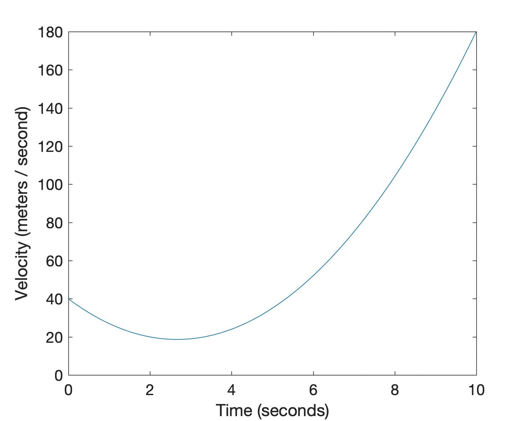
Notice that the car retains a positive velocity throughout the journey, and this is because it never changes direction. Hence, if we had to imagine ourselves sitting in this moving car, the speedometer would be showing us the values that we have just plotted on the velocity graph (since the velocity remains positive throughout, otherwise we would have to find the absolute value of the velocity to work out the speed). If we had to apply the power rule to y(t) to find its derivative, then we would find that the velocity is defined by the following function:
v(t) = y’(t) = 3t2 – 16t + 40
We can also plot the acceleration graph:
We find that the graph is now characterised by negative acceleration in the time interval, t = [0, 2.7) seconds. This is because acceleration is the derivative of velocity, and within this time interval the car’s velocity is decreasing. If we had to, again, apply the power rule to v(t) to find its derivative, then we would find that the acceleration is defined by the following function:
a(t) = v’(t) = 6t – 16
Putting all functions together, we have the following:
y(t) = t3 – 8t2 + 40t
v(t) = y’(t) = 3t2 – 16t + 40
a(t) = v’(t) = 6t – 16
If we substitute for t = 10s, we can use these three functions to find that by the end of the journey, the car has travelled 600m, its velocity is 180 m/s, and it is accelerating at 44 m/s2. We can verify that all of these values tally with the graphs that we have just plotted.
We have framed this particular example within the context of finding a car’s velocity and acceleration. But there is a plethora of real-life phenomena that change with time (or variables other than time), which can be studied by applying the concept of derivatives as we have just done for this particular example. To name a few:
Growth rate of a population (be it a collection of humans, or a colony of bacteria) over time, which can be used to predict changes in population size in the near future.
Changes in temperature as a function of location, which can be used for weather forecasting.
Fluctuations of the stock market over time, which can be used to predict future stock market behaviour.
Derivatives also provide salient information in solving optimization problems, as we shall be seeing next.
Applications of Derivatives in Optimization Algorithms
We had already seen that an optimization algorithm, such as gradient descent, seeks to reach the global minimum of an error (or cost) function by applying the use of derivatives.
Let’s take a closer look at what the derivatives tell us about the error function, by going through the same exercise as we have done for the car example.
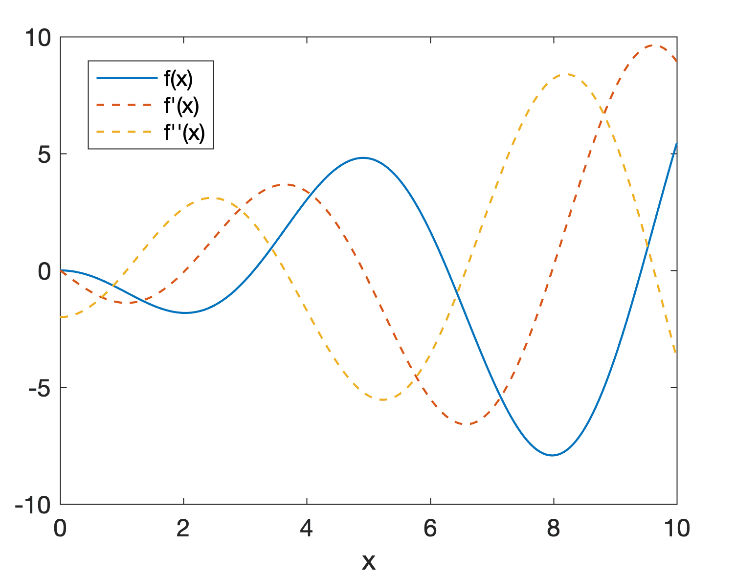
For this purpose, let’s consider the following one-dimensional test function for function optimization:
f(x) = –x sin(x)
We can apply the product rule to f(x) to find its first derivative, denoted by f’(x), and then again apply the product rule to f’(x) to find the second derivative, denoted by f’’(x):
f’(x) = -sin(x) – x cos(x)
f’’(x) = x sin(x) – 2 cos(x)
We can plot these three functions for different values of x to visualize them:
Similar to what we have observed earlier for the car example, the graph of the first derivative indicates how f(x) is changing and by how much. For example, a positive derivative indicates that f(x) is an increasing function, whereas a negative derivative tells us that f(x) is now decreasing. Hence, if in its search for a function minimum, the optimization algorithm performs small changes to the input based on its learning rate, ε:
x_new = x – ε f’(x)
Then the algorithm can reduce f(x) by moving to the opposite direction (by inverting the sign) of the derivative.
We might also be interested in finding the second derivative of a function.
We can think of the second derivative as measuring curvature.
– Page 86, Deep Learning, 2017.
For example, if the algorithm arrives at a critical point at which the first derivative is zero, it cannot distinguish between this point being a local maximum, a local minimum, a saddle point or a flat region based on f’(x) alone. However, when the second derivative intervenes, the algorithm can tell that the critical point in question is a local minimum if the second derivative is greater than zero. For a local maximum, the second derivative is smaller than zero. Hence, the second derivative can inform the optimization algorithm on which direction to move. Unfortunately, this test remains inconclusive for saddle points and flat regions, for which the second derivative is zero in both cases.
Optimization algorithms based on gradient descent do not make use of second order derivatives and are, therefore, known as first-order optimization algorithms. Optimization algorithms, such as Newton’s method, that exploit the use of second derivatives, are otherwise called second-order optimization algorithms.
Further Reading
This section provides more resources on the topic if you are looking to go deeper.
Books
Calculus for Dummies, 2016.
Infinite Powers, 2020.
Deep Learning, 2017.
Algorithms for Optimization, 2019.
Summary
In this tutorial, you discovered different applications of derivatives.
Specifically, you learned:
The use of derivatives can be applied to real-life problems that we find around us.
The use of derivatives is essential in machine learning, for function optimization.
Do you have any questions?
Ask your questions in the comments below and I will do my best to answer.
The post Applications of Derivatives appeared first on Machine Learning Mastery.
Read MoreMachine Learning Mastery