A Gentle Introduction to Multivariate Calculus

It is often desirable to study functions that depend on many variables. 

Multivariate calculus provides us with the tools to do so by extending the concepts that we find in calculus, such as the computation of the rate of change, to multiple variables. It plays an essential role in the process of training a neural network, where the gradient is used extensively to update the model parameters. 

In this tutorial, you will discover a gentle introduction to multivariate calculus. 

After completing this tutorial, you will know:

A multivariate function depends on several input variables to produce an output. 
The gradient of a multivariate function is computed by finding the derivative of the function in different directions. 
Multivariate calculus is used extensively in neural networks to update the model parameters. 

Let’s get started. 

Tutorial Overview

This tutorial is divided into three parts; they are:

Re-Visiting the Concept of a Function 
Derivatives of Multi-Variate Functions
Application of Multivariate Calculus in Machine Learning

Re-Visiting the Concept of a Function

We have already familiarised ourselves with the concept of a function, as a rule that defines the relationship between a dependent variable and an independent variable. We have seen that a function is often represented by y = f(x), where both the input (or the independent variable), x, and the output (or the dependent variable), y, are single real numbers. 

Such a function that takes a single, independent variable and defines a one-to-one mapping between the input and output, is called a univariate function. 

For example, let’s say that we are attempting to forecast the weather based on the temperature alone. In this case, the weather is the dependent variable that we are trying to forecast, which is a function of the temperature as the input variable. Such a problem can, therefore, be easily framed into a univariate function. 

However, let’s say that we now want to base our weather forecast on the humidity level and the wind speed too, in addition to the temperature. We cannot do so by means of a univariate function, where the output depends solely on a single input. 

Hence, we turn our attention to multivariate functions, so called because these functions can take several variables as input. 

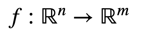
Formally, we can express a multivariate function as a mapping between several real input variables, n, to a real output:

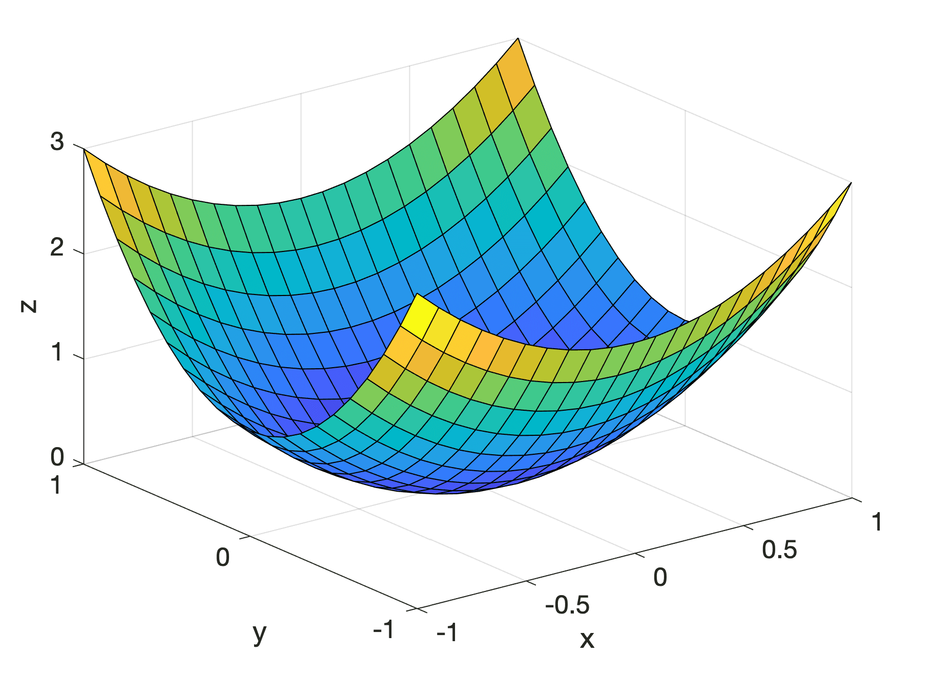
For example, consider the following parabolic surface:

f(x, y) = x2 + 2y2

This is a multivariate function that takes two variables, x and y, as input, hence n = 2, to produce an output. We can visualise it by graphing its values for x and y between -1 and 1.

Similarly, we can have multivariate functions that take more variables as input. Visualising them, however, may be difficult due to the number of dimensions involved. 

We can even generalize the concept of a function further by considering functions that map multiple inputs, n,  to multiple outputs, m:

These functions are more often referred to as vector-valued functions. 

Derivatives of Multi-Variate Functions

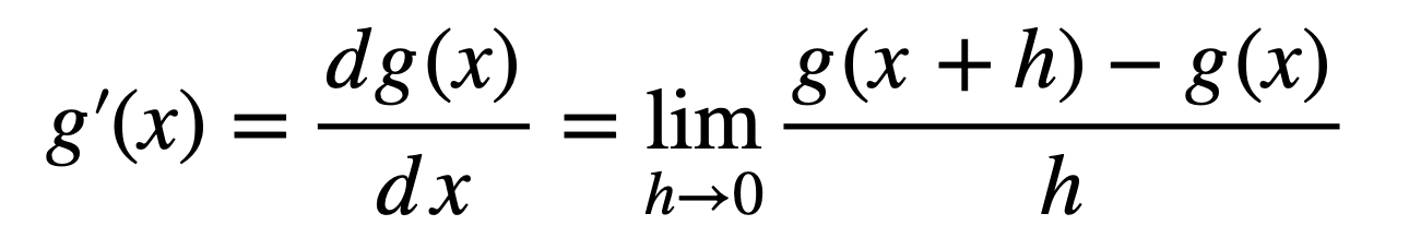
Recall that calculus is concerned with the study of the rate of change. For some univariate function, g(x), this can be achieved by computing its derivative:

The generalization of the derivative to functions of several variables is the gradient. 

– Page 146, Mathematics of Machine Learning, 2020.

The technique to finding the gradient of a function of several variables involves varying each one of the variables at a time, while keeping the others constant. In this manner, we would be taking the partial derivative of our multivariate function with respect to each variable, each time. 

The gradient is then the collection of these partial derivatives. 

– Page 146, Mathematics of Machine Learning, 2020.

In order to visualize this technique better, let’s start off by considering a simple univariate quadratic function of the form:

g(x) = x2

Finding the derivative of this function at some point, x, requires the application of the equation for g’(x) that we have defined earlier. We can, alternatively, take a shortcut by using the power rule to find that:

g’(x) = 2x

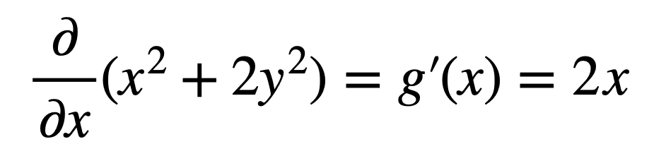
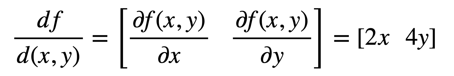
Furthermore, if we had to imagine slicing open the parabolic surface considered earlier, with a plane passing through y = 0, we realise that the resulting cross-section of f(x, y) is the quadratic curve, g(x) = x2. Hence, we can calculate the derivative (or the steepness, or slope) of the parabolic surface in the direction of x, by taking the derivative of f(x, y) but keeping y constant. We refer to this as the partial derivative of f(x, y) with respect to x, and denote it by ∂ to signify that there are more variables in addition to x but these are not being considered for the time being. Therefore, the partial derivative with respect to x of f(x, y) is:

We can similarly hold x constant (or, in other words, find the cross-section of the parabolic surface by slicing it with a plane passing through a constant value of x) to find the partial derivative of f(x, y) with respect to y, as follows:

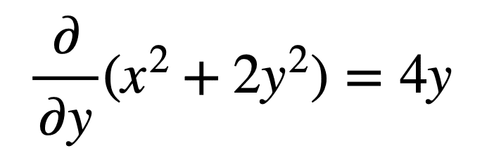
What we have essentially done is that we have found the univariate derivative of f(x, y) in  each of the x and y directions. Combining the two univariate derivatives as the final step, gives us the multivariate derivative (or the gradient):

The same technique remains valid for functions of higher dimensions. 

Application of Multivariate Calculus in Machine Learning

Partial derivatives are used extensively in neural networks to update the model parameters (or weights). 

We had seen that, in minimizing some error function, an optimization algorithm will seek to follow its gradient downhill. If this error function was univariate, and hence a function of a single independent weight, then optimizing it would simply involve computing its univariate derivative.

However, a neural network comprises many weights (each attributed to a different neuron) of which the error is a function. Hence, updating the weight values requires that the gradient of the error curve is calculated with respect to all of these weights. 

This is where the application of multivariate calculus comes into play. 

The gradient of the error curve is calculated by finding the partial derivative of the error with respect to each weight; or in other terms, finding the derivative of the error function by keeping all weights constant except the one under consideration. This allows each weight to be updated independently of the others, to reach the goal of finding an optimal set of weights. 

Further Reading

This section provides more resources on the topic if you are looking to go deeper.

Books

Single and Multivariable Calculus, 2020.
Mathematics for Machine Learning, 2020.
Algorithms for Optimization, 2019.
Deep Learning, 2019.

Summary

In this tutorial, you discovered a gentle introduction to multivariate calculus.

Specifically, you learned:

A multivariate function depends on several input variables to produce an output. 
The gradient of a multivariate function is computed by finding the derivative of the function in different directions. 
Multivariate calculus is used extensively in neural networks to update the model parameters. 

Do you have any questions?
Ask your questions in the comments below and I will do my best to answer.

The post A Gentle Introduction to Multivariate Calculus appeared first on Machine Learning Mastery.

Read MoreMachine Learning Mastery