

Non-small cell lung cancer (NSCLC) is the most common type of lung cancer, and is composed of tumors with significant molecular heterogeneity resulting from differences in intrinsic oncogenic signaling pathways [1]. Enabling precision medicine, anticipating patient preferences, detecting disease, and improving care quality for NSCLC patients are important topics among healthcare and life sciences (HCLS) communities.
Applying machine learning (ML) to diverse health datasets, known as multimodal machine learning (multimodal ML), is an active area of research and development. Analyzing linked patient-level data from diverse data modalities, such as genomics and medical imaging, promises to accelerate improvements in patient care. However, performing analyses of multiple modalities at scale has been challenging in on-premises or cloud environments due to the distinct infrastructure requirements of each modality. With Amazon SageMaker, you can create purpose-built pipelines and scale them to meet your needs easily, paying only for what you use.
We’re announcing a new solution on lung cancer survival prediction in Amazon SageMaker JumpStart, based on the blog posts Building Scalable Machine Learning Pipelines for Multimodal Health Data on AWS and Training Machine Learning Models on Multimodal Health Data with Amazon SageMaker. JumpStart provides pre-trained, open-source models and pre-built solution templates for a wide range of problem types to help data scientists and ML practitioners get started on training and deploying ML models quickly. This is the first HCLS solution offered by JumpStart.
The solution builds a multimodal ML model for predicting survival outcome of patients diagnosed with NSCLC. The multimodal model is trained on data derived from different modalities or domains, including medical imaging, genomic, and clinical data. Multimodal ML has been adopted in HCLS for personalized treatment, clinical decision support, and drug response prediction. In this post, we demonstrate how you can create a scalable, purpose-built ML pipeline easily with one-click deployment from JumpStart.
What’s in the dataset
Non–small cell lung cancer is the leading cause for cancer death [2]. However, no two cancer diagnoses are alike, because tumors contain significant molecular heterogeneity resulting from differences in intrinsic oncogenic signaling pathways [1]. In addition, different clinical information collected from patients may impact prognosis and treatment options. Therefore, enabling precision medicine, anticipating patient preferences, detecting disease, and improving care quality for NSCLC patients is of utmost importance in the oncology and HCLS communities.
The Non-Small Cell Lung Cancer (NSCLC) Radiogenomic dataset [3] comprises medical imaging, clinical, and genomic data collected from a cohort of early-stage NSCLC patients referred for surgical treatment. It includes Computed Tomography (CT), Positron Emission Tomography (PET)/CT images, semantic annotations of the tumors as observed on the medical images using a controlled vocabulary, segmentation maps of tumors in the CT scans, and quantitative values obtained from the PET/CT scans. The genomic data contains gene mutation and RNA sequencing data from samples of surgically excised tumor tissue. It also consists of clinical data reflective of electronic health records (EHR) such as age, gender, weight, ethnicity, smoking status, Tumor Node Metastasis (TNM) stage, histopathological grade, and survival outcome. Each data modality presents a different view of a patient.
Medical imaging data
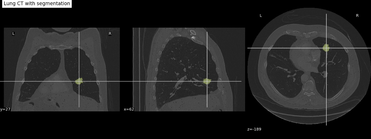
Medical imaging biomarkers of cancer promise improvements in patient care through advances in precision medicine. Compared to genomic biomarkers, imaging biomarkers provide the advantages of being non-invasive, and characterizing a heterogeneous tumor in its entirety, as opposed to limited tissue available via biopsy [3]. In this dataset, CT and PET/CT imaging sequences were acquired for patients prior to surgical procedures. Segmentation of tumor regions were annotated by two expert thoracic radiologists. The following image is an example overlay of a tumor segmentation onto a lung CT scan (case R01-093 in the dataset).
Genomic data
Samples of surgically excised tumor tissues were analyzed with RNA sequencing technology. The dataset file that is available from the source was preprocessed using open-source tools, including STAR v.2.3 for alignment and Cufflinks v.2.0.2 for expression calls [4]. The original dataset (GSE103584_R01_NSCLC_RNAseq.txt.gz) can be found on the NCBI website. Although the original data contains more than 22,000 genes, for the purpose of demonstration, we used 21 genes from 10 highly co-expressed gene clusters (metagenes) that were identified, validated in publicly available gene-expression cohorts, and correlated with prognosis [4].
The following table shows the tabular representation of the gene expression data. Each row corresponds to a patient, and the columns represent a subset of genes selected for demonstration. The value denotes the expression level of a gene for a patient. A higher value means the corresponding gene is highly expressed in that specific tumor sample.
Case_ID
LRIG1
HPGD
GDF15
CDH2
POSTN
……
R01-024
26.7037
3.12635
13.0269
0
36.4332
……
R01-153
15.2133
5.0693
0.90866
0
32.8595
……
R01-031
5.54082
1.23083
29.8832
1.13549
34.8544
……
R01-032
12.8391
7.21931
12.0701
0
7.77297
……
R01-033
33.7975
3.19058
5.43418
0
9.84029
……
Clinical data
Clinical data was collected from medical records. It included demographics, smoking history, survival, recurrence status, histology, histopathological grading, Pathological TNM staging, and survival outcome of patients. The data is stored in CSV format, as shown in the following table.
Case ID
Survival Status
Age at Histological Diagnosis
Weight (lbs)
Smoking status
Pack Years
Quit Smoking Year
Chemotherapy
Adjuvant Treatment
EGFR mutation status
……
R01-005
Dead
84
145
Former
20
1951
No
No
Wildtype
……
R01-006
Alive
62
Not Collected
Former
Not Collected
nan
No
No
Wildtype
……
R01-007
Dead
68
Not Collected
Former
15
1968
Yes
Yes
Wildtype
……
R01-008
Alive
73
102
Nonsmoker
nan
nan
No
No
Wildtype
……
R01-009
Dead
59
133
Current
100
nan
No
……
……
……
Solution overview
Working with multimodal healthcare data for ML purposes often requires dedicated data processing pipelines and compute resources to extract relevant biomarkers and features. Collecting, storing, and managing extracted features can be challenging. In this JumpStart solution, we show you how to process each modality in separate notebooks, use Amazon SageMaker Processing for compute intensive 3D image construction, use Amazon SageMaker Feature Store to centrally store extracted features for ML modeling, run SageMaker experiments to enhance ML lineage, implement the SageMaker built-in algorithm to train an ML model without sophisticated coding, and deploy a model for real-time prediction with SageMaker deployment.
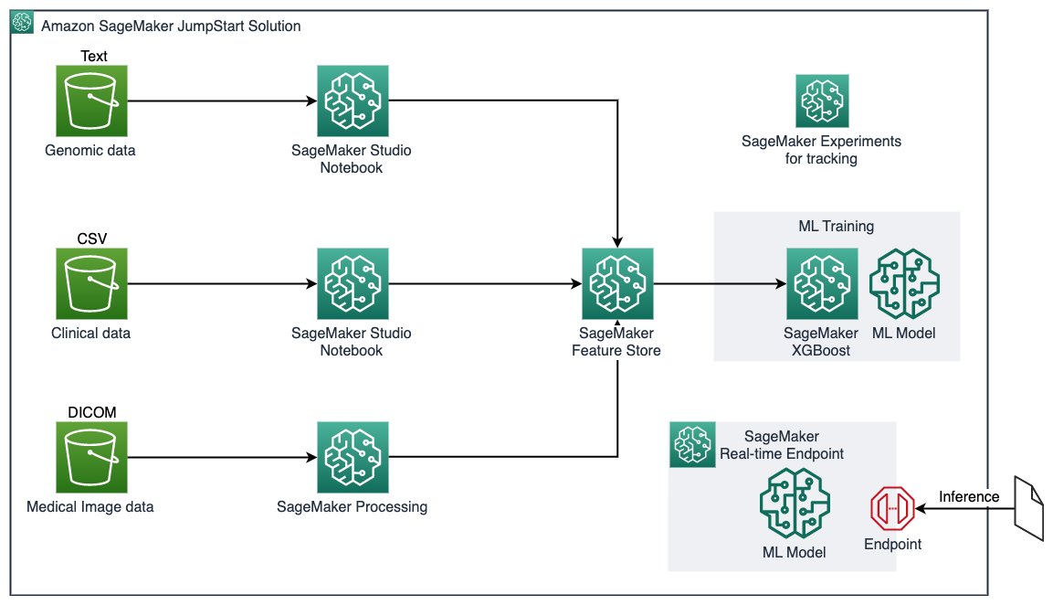
The architecture for the solution is illustrated in the following diagram.
The key services involved are as follows:
Amazon SageMaker JumpStart – JumpStart provides pre-trained, open-source models for a wide range of problem types to help you get started. JumpStart also provides solution templates that set up infrastructure for common use cases, and notebooks for ML with SageMaker. This service is where we launch our solution.
Amazon Simple Storage Service – Amazon S3 is an object storage service that offers scalability, data availability, security, and performance. Amazon S3 allows you to store data to be used by SageMaker.
Amazon SageMaker Studio notebooks – You can launch these collaborative notebooks quickly because you don’t need to set up compute instances and file storage beforehand. This is the environment you can build in.
SageMaker Processing jobs – These jobs enable you to analyze data and evaluate ML models. This managed experience helps you run your data processing workloads, such as feature engineering, data validation, and model interpretation. This service allows you to process the data that is stored in Amazon S3.
Amazon SageMaker Feature Store – You can create, share, and manage features for ML development. This is where you store processed features to use for training.
Amazon SageMaker Experiments – You can organize, track, compare, and evaluate ML experiments.
Built-in XGBoost algorithm (eXtreme gradient boosting) – This is a popular and efficient open-source implementation of the gradient boosting algorithm that is used for training the.
SageMaker training jobs – You create a managed training job in SageMaker using four attributes: the URL of the S3 bucket you’ve stored the training data, compute resources, the URL of the S3 bucket where you want to store the output of the job, and the Amazon Elastic Container Registry (Amazon ECR) path where the training code is stored.
SageMaker real-time endpoints – These endpoints are ideal for inference workloads where you have real-time, interactive, low-latency requirements. You deploy the model to SageMaker hosting services and get an endpoint that can be used for inference.
With this JumpStart solution, you can easily spin up the solution in Amazon SageMaker Studio, and follow the post to explore, train, and deploy a lung cancer survival status prediction model for learning purposes.
Prerequisites
To use the Lung Cancer Survival Prediction solution provided by JumpStart, you need to have a Studio domain. A SageMaker project and JumpStart must also be enabled.
If you don’t have a Studio domain, refer to Onboard to Amazon SageMaker Domain Using Quick Setup.
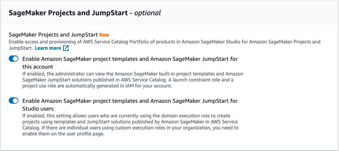
If you have a SageMaker domain, make sure that the project and JumpStart features have been enabled by following these steps:
On the SageMaker console, choose the gear icon next to Domain.
Choose Next.
In the SageMaker Projects and JumpStart section, select Enable Amazon SageMaker project templates and Amazon SageMaker JumpStart for this account and Enable Amazon SageMaker project templates and Amazon SageMaker JumpStart for Studio users.
We have completed the prerequisites needed to use JumpStart.
Deploy the solution and example demo notebook
To start using the Lung Cancer Survival Prediction solution, complete the following steps:
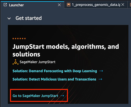
Open Studio.
Choose Go to SageMaker JumpStart under Jumpstart models, algorithms, and solutions.
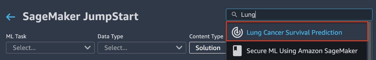
To find the solution within JumpStart, choose Explore All Solutions.
Search for and choose Lung Cancer Survival Prediction.
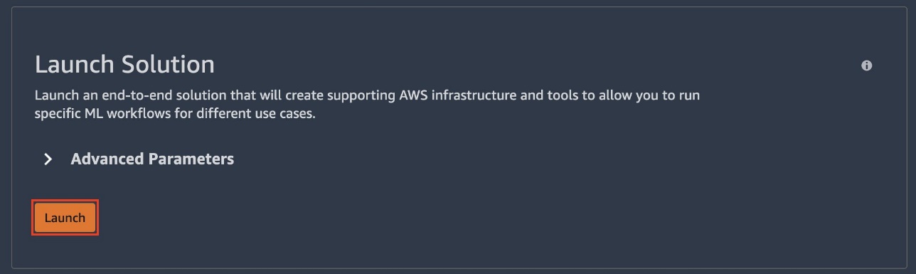
Under Launch Solution, choose Launch.
Note that you can specify custom execution roles to be used throughout this solution, otherwise execution roles are created for you.
It should take a few moments for the solution to launch. You can follow along as a number of resources are launched.
Wait until the endpoint and model statuses show as Complete. You may need to refresh the page.
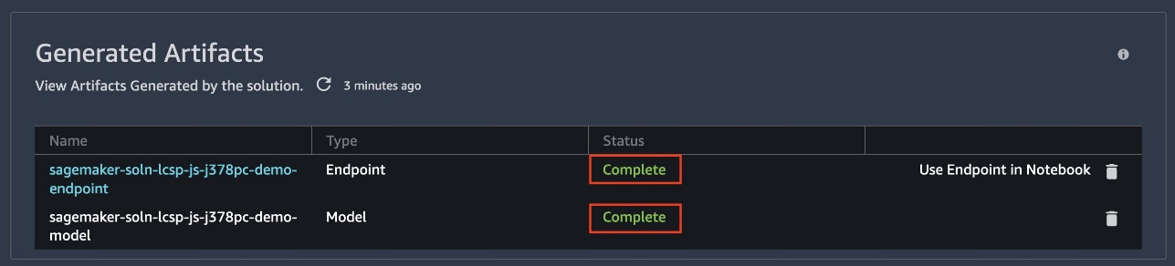
This solution generates a model, endpoint configuration, endpoint, and five notebooks.
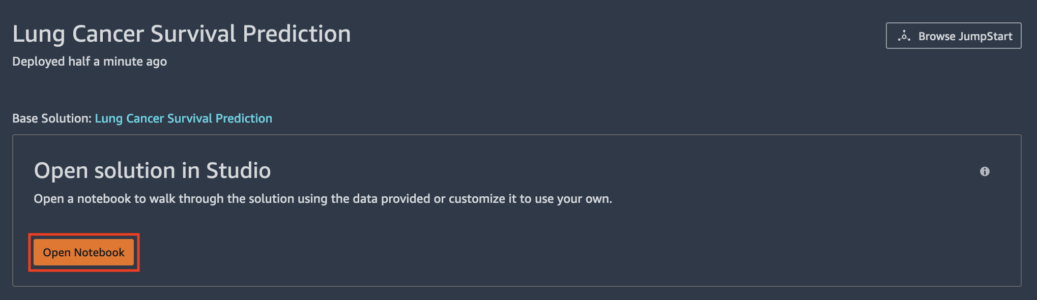
To navigate to the first notebook, under Open solution in Studio, choose Open Notebook.
To navigate to other notebooks, select the folder icon and open the S3Downloads folder.
Open the jumpstart-prod-lcsp_****** folder.
Form here, you can access the following notebooks:
0_demo.ipynb – Demonstrates how to send inference requests to a pre-deployed endpoint and receive a model response.
1_preprocess_genomic_data.ipynb – Showcases how to read and process genomic data (in tabular format).
2_preprocess_clinical_data.ipynb – Demonstrates how to read and process health insurance claims data (in tabular format).
3_preprocess_imaging_data.ipynb – Showcases how to read and process medical imagining data in DICOM file format and convert to NIfTI neuroimaging format. Therefore, it takes medical imagining data in volumetric format. Note that in notebooks 1, 2, and 3, we store the output of each processing job in Feature Store.
4_train_test_model.ipynb – Demonstrates how to access multimodal features from Feature Store, train an XGBoost model, and predict the survival status of patients diagnosed with non-small cell lung cancer.
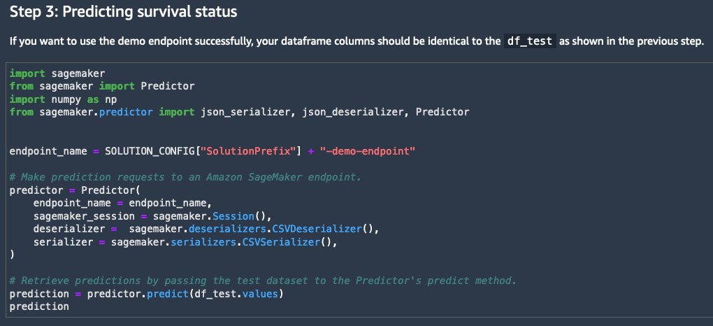
After the solution is deployed in Studio, you can start building a lung cancer survival status prediction using multimodal health data. To start, let’s look at the 0_demo.ipynb notebook, which demonstrates how to send inference requests to a pre-deployed endpoint, and get the model response (survived vs. dead).
In this notebook, you can see a preview of the datasets (which we cover in a later section), and the steps needed to make predictions with an endpoint that has already been deployed. A predictor is instantiated to begin making real-time predictions against a SageMaker endpoint. We can use the predictor’s predict function to invoke the endpoint with test data.
The endpoint returns the predicted survival status, which is used to assess model performance, as shown in the following screenshot.
Feature engineering
As described earlier, genomic, clinical, and medical imaging data is available in the NSCLC dataset for us to create a comprehensive view of a patient. To process and compute the features that later help us build a ML model, let’s start with the genomic data pipeline in 1_preprocess_genomic_data.ipynb and step through 2_preprocess_clinical_data.ipynb and 3_preprocess_imaging_data.ipynb for the clinical data pipeline and medical imaging pipeline, respectively.
Genomic
For genomic data, we read the RNA sequence data from the JumpStart solution bucket into the notebook 1_preprocess_genomic_data.ipynb:
We then keep 21 genes from 10 highly co-expressed gene clusters (metagenes) that were identified, validated in publicly available gene-expression cohorts, and correlated with prognosis [4]:
With the genomic features ready for analysis, we ingest the features into Feature Store as a feature group. Having the features in the Feature Store allows us to repeatedly source the important genomic features in the downstream analysis with governance.
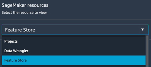
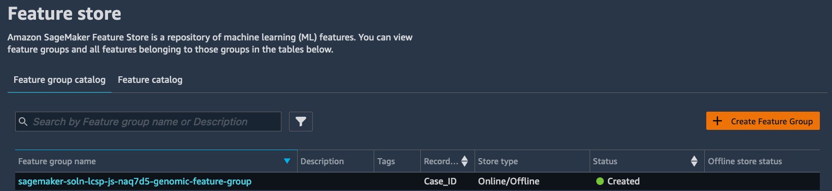
To see the recently ingested features in the Feature Store UI, under SageMaker resources, choose Feature Store.
From here, you can find the most recently ingested features into Feature Store. The feature group name should be sagemaker-soln-lcsp-js-******-genomic-feature-group.
Clinical
For clinical data, we perform data cleaning and processing on the data hosted on the JumpStart solution bucket and ingest into the Feature Store, as shown in 2_preprocess_clinical_data.ipynb:
We run one-hot encoding to convert categorical attributes to numerical attributes. We then remove columns that don’t provide useful information (such as dates), and remove rows with missing values. Afterwards, we create another feature group in Feature Store to store the clinical features, similarly to how we did in the genomic notebook.
Medical imaging
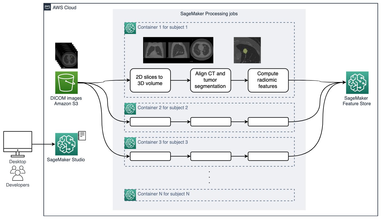
For medical imaging data, we create patient-level 3-dimensional radiomic features that explain the size, shape, and visual attributes of the tumors observed in the CT scans, and store them in a feature group in Feature Store. For each patient study, the following steps are performed. Details can be found in 3_preprocess_imaging_data.ipynb.
Read the 2D DICOM slice files for both the CT scan and tumor segmentation, combine them to 3D volumes, and save the volumes in NIfTI format.
Align CT volume and tumor segmentation so we can focus the computation inside the tumor.
Compute radiomic features describing the tumor region using the pyradiomics library. We extract 120 radiomic features of eight classes such as statistical representations of the distribution and co-occurrence of the intensity within the tumorous region of interest, and shape-based measurements describing the tumor morphologically.
It’s worth mentioning how the medical imaging pipeline is done at scale. Processing hundreds of large, high-resolution 3D images requires the right compute resource. Parallelizing the tasks can further reduce the total processing time and help you get the results sooner. We use SageMaker Processing, an on-demand, scalable feature for data processing need in SageMaker, to run DICOM to 3D volume construction, CT/tumor segmentation alignment, radiomic feature extract, and feature store ingestion. We parallelize the processing to one job per patient data, as shown in the following figure.
To launch the SageMaker Processing jobs for multiple patients in parallel efficiently, we run the utility function launch_processing_job(), which submits a configured SageMaker Processing job on one ml.r5.large instance, in a for loop.
In this case, we need to work with the service quota for the instance cleverly. The default service quota for the number of instances across processing jobs and number of ml.r5.large instances is four. If your account has a higher limit, you may run a higher number of simultaneous processing jobs (therefore a faster completion time). To request a quota increase, refer to AWS service quotas. We implemented the function wait_for_instance_quota() to check for the current job count that is in InProgress state and limit the total count in this experiment to the value set in job_limit. If the total running job count is at the limit, the function waits the number of seconds specified in the wait argument and checks the job count again. This is to account for the account-level SageMaker quota that may cause errors in the for loop.
Another challenge when we work with a large amount of processing and training jobs is keeping track of the details and the lineage of all the jobs in an experiment. We use SageMaker Experiments to achieve this. Setting up the experiment tracking is simple. When each SageMaker Processing job is submitted within launch_processing_job(), an experiment configuration is set up and is provided to run the job. See the following code:
We can then find the status and details of each job on the Experiments and trials menu.
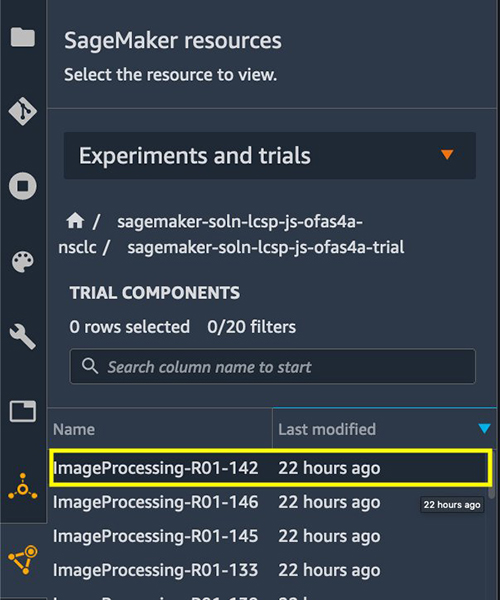
Note that medical imaging processing and feature store offline store synchronization takes some time to complete for all patients, and imaging features may not be available in the offline store immediately for model training in the next section. To make sure the medical imaging features are available for training, a check of total entry count is implemented before proceeding to the next notebook 4_train_test_model.ipynb.
Modeling
As described earlier, we process the data of each modality in three separate notebooks, and create and ingest features into per-modality feature groups. At the time of training, we flexibly choose multimodal features using a SQL query against the offline store in Feature Store. We then preprocess the data and apply dimensionality reduction prior to training an XGBoost model from the SageMaker built-in algorithm for the binary classification task of predicting the survival outcome of patients. After the model is trained, we host the XGBoost model in a SageMaker real-time endpoint for testing and inference purposes.
To create a multimodal view of a patient for model training, we join the feature vectors from three modalities. This includes the following steps:
Normalize the range of independent features using feature scaling.
For ML training, run a query against the three feature groups to join the data stored in the offline store. For the given dataset, this integration results in 119 data samples, where each sample is a 215-dimensional vector.
Perform principal component analysis (PCA) on the features to reduce the dimensionality and identify the most discriminative features that contribute to 95% variance in the data. This results in a dimensionality reduction from 215 features down to 45 principal components, which constitute features for the supervised learner.
Randomly shuffle this data and divide it into 80% for training and 20% for testing the model.
Further split the training data into 80% for training and 20% for validating the model.
To train the ML model, construct an estimator of the gradient boosting library XGBoost through a SageMaker XGBoost container. Because our objective is to train a baseline model with multimodal data, we consider default hyperparameters and don’t perform any hyperparameter tuning. The model predicts NSCLC patients’ survival status (dead or alive) in a form of probability. In addition to the model and prediction, we also generate reports to explain the model. The medical imaging pipeline produces 3D lung CT volumes and tumor segmentation for visualization purposes. See the following code
After we train the model, we can deploy the model to a SageMaker endpoint to give us the ability to make predictions in real time in the next step.
Inference
To deploy the endpoint, we use the deploy() method from the trained estimator. The deploy method uses several parameters. We provide the deploy method with an instance_count, which specifies the number of compute instances to launch initially, and instance_type, which specifies the compute instance type. We then use a CSVSerilizer to serialize the incoming data of various formats to a CSV-formatted string for our endpoint. See the following code:
After the endpoint has been deployed, we can make requests and receive predictions in real time. To make predictions, we use the predict() method to pass in data from the test_data data frame:
The predictor returns a probability. If the probability is greater than 0.5, the patient is less likely to survive NSCLC. If the probability is less than 0.5, the patient is more likely to survive NSCLC.
Finally, we evaluate the prediction with the ground truth in the test_data using accuracy, F1 score, precision, recall, and a confusion matrix. We see that the model can accurately predict 19 out of 25 patients in the test_data, with a balanced precision and recall (and F1 score).
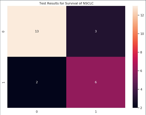
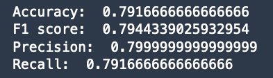
Clean up
After completing this solution, we delete resources instantiated from the solution to avoid incurring further charges. To delete the endpoint and model resources, run the Clean up step in 4_train_test_model.ipynb.
To delete the full JumpStart solution, go to the launched solution you deployed by choosing the JumpStart icon. Under Your launched solutions, select Lung Cancer Survival Prediction, and scroll to the bottom of the solution page. Under Delete solution, choose Delete all resources. This will delete the launched resources including the notebooks that were created.
If you now go back to the S3Downloads folder, you will notice that the Studio notebooks have been deleted.
To delete your SageMaker domain, refer to Delete an Amazon SageMaker Domain.
Conclusion
In this post, we announced a new JumpStart solution that predicts the survival status of non-small cell lung cancer patients using multimodal data. We walked you through the diverse multimodal dataset (medical imaging, genomic, and clinical records); discussed our solution that uses SageMaker features such as SageMaker Processing, Feature Store, the built-in XGBoost algorithm, and SageMaker real-time endpoints; and showed you how to easily run the solution in JumpStart, where cloud resources are managed and deployed for you with just one click.
We encourage you to launch the solution in Studio and step through the notebooks in detail to learn how to process complex healthcare multimodal data, build a survival status prediction model, and make inference on the data using SageMaker. You will then have the knowledge to build an ML solution using SageMaker for your own healthcare and life sciences datasets and use cases.
To learn more about other solutions, pre-built models, and algorithms in JumpStart, visit SageMaker JumpStart.
To learn more about multimodal and multi-omics analysis on AWS, visit Simplifying Multi-modal & Multi-omics Analysis with AWS for Health.
Disclaimer
This solution is for demonstrative purposes only. It is not for clinical use and is not a substitute for professional medical advice, diagnosis, or treatment. The associated notebooks, including the trained model and sample data, are not intended for production. It is each customers’ responsibility to determine whether they are subject to HIPAA, and if so, how best to comply with HIPAA and its implementing regulations. Before using AWS in connection with protected health information, customers must enter an AWS Business Associate Addendum (BAA) and follow its configuration requirements.
References
[1] Travis, William D., et al. “The 2015 World Health Organization classification of lung tumors: impact of genetic, clinical and radiologic advances since the 2004 classification.” Journal of thoracic oncology 10.9 (2015): 1243-1260.
[2] Jernal, A., et al. “Cancer statistics, 2002.” CA cancer J clin52.1 (2002): 23-47.
[3] Bakr, Shaimaa, et al. “A radiogenomic dataset of non-small cell lung cancer.” Scientific data 5.1 (2018): 1-9.
[4] Zhou, Mu, et al. “Non–small cell lung cancer radiogenomics map identifies relationships between molecular and imaging phenotypes with prognostic implications.” Radiology 286.1 (2018): 307.
About the Authors
Michael Hsieh is a Principal AI/ML Specialist Solutions Architect. He focuses on solving business challenges using AI/ML for customers in the healthcare and life sciences industry. As a Seattle transplant, he loves exploring the great Mother Nature the city has to offer, such as the hiking trails, scenery kayaking in the SLU, and the sunset at Shilshole Bay. As a former long-time resident of Philadelphia, he has been rooting for the Philadelphia Eagles and Philadelphia Phillies.
Olivia Choudhury, PhD, is a Senior Partner Solutions Architect at AWS. She helps partners in the healthcare and life sciences domain design, develop, and scale state-of-the-art solutions using AWS. She has a background in genomics, healthcare analytics, federated learning, and privacy-preserving machine learning. Outside of work, she plays board games, paints landscapes, and collects manga.
Curt Lockhart is an AI/ML Specialist Solutions Architect at AWS. He comes from a non-traditional background of working in the arts before his move to tech, and enjoys making machine learning approachable for each customer. Based in Seattle, you can find him venturing to local art museums, catching a concert, and wandering throughout the cities and outdoors of the Pacific Northwest.
Read MoreAWS Machine Learning Blog