

In recent years, social media has become a common means for sharing and consuming news. However, the spread of misinformation and fake news on these platforms has posed a major challenge to the well-being of individuals and societies. Therefore, it is imperative that we develop robust and automated solutions for early detection of fake news on social media. Traditional approaches rely purely on the news content (using natural language processing) to mark information as real or fake. However, the social context in which the news is published and shared can provide additional insights into the nature of fake news on social media and improve the predictive capabilities of fake news detection tools. In this post, we demonstrate how to use Amazon Neptune ML to detect fake news based on the content and social context of the news on social media.
Neptune ML is a new capability of Amazon Neptune that uses graph neural networks (GNNs), a machine learning (ML) technique purpose-built for graphs, to make easy, fast, and accurate predictions using graph data. Making accurate predictions on graphs with billions of relationships requires expertise. Existing ML approaches such as XGBoost can’t operate effectively on graphs because they’re designed for tabular data. As a result, using these methods on graphs can take time, require specialized skills, and produce suboptimal predictions.
Neptune ML uses the Deep Graph Library (DGL), an open-source library to which AWS contributes, and Amazon SageMaker to build and train GNNs, including Relational Graph Convolutional Networks (R-GCNs) for tasks such as node classification, node regression, link prediction, or edge classification.
The DGL makes it easy to apply deep learning to graph data, and Neptune ML automates the heavy lifting of selecting and training the best ML model for graph data. It provides fast and memory-efficient message passing primitives for training GNNs. Neptune ML uses the DGL to automatically choose and train the best ML model for your workload. This enables you to make ML-based predictions on graph data in hours instead of weeks. For more information, see Amazon Neptune ML for machine learning on graphs.
Amazon SageMaker is a fully managed service that provides every developer and data scientist with the ability to prepare, build, train, and deploy ML models quickly.
Overview of GNNs
GNNs are neural networks that take graphs as input. These models operate on the relational information in data to produce insights not possible in other neural network architectures and algorithms. A graph (sometimes called a network) is a data structure that highlights the relationships between components in the data. It consists of nodes (or vertices) and edges (or links) that act as connections between the nodes. Such a data structure has an advantage when dealing with entities that have multiple relationships. Graph data structures have been around for centuries, with a wide variety of modern use cases.
GNNs are emerging as an important class of deep learning (DL) models. GNNs learn embeddings on nodes, edges, and graphs. GNNs have been around for about 20 years, but interest in them has dramatically increased in the last 5 years. In this time, we’ve seen new architectures emerge, novel applications realized, and new platforms and libraries enter the scene. There are several potential research and industry use cases for GNNs, including the following:
Computer vision – Generating scene graphs
Forecasting – Predicting traffic volume
Node classification – Implementing targeted campaigns, detecting fake news
Graph classification – Predicting the properties of a chemical compound
Link prediction – Building recommendation systems
Other – Predicting adversarial attacks
Dataset
For this post, we use the BuzzFeed dataset from the 2018 version of FakeNewsNet. The BuzzFeed dataset consists of a sample of news articles shared on Facebook from nine news agencies over 1 week leading up to the 2016 US election. Every post and the corresponding news article have been fact-checked by BuzzFeed journalists. The following table summarizes key statistics about the BuzzFeed dataset from FakeNewsNet.
Category
Amount
Users
15,257
Authors
126
Publishers
28
Social Links
634,750
Engagements
25,240
News Articles
182
Fake News
91
Real News
91
To get the raw data, you can complete the following steps:
Clone the FakeNewsNet repository from GitHub.
Check out the old version branch.
Change the directory to Data/BuzzFeed.
Each row in the Users.txt file provides a UUID for the corresponding user.
Each row in the News.txt file provides a name and ID for the corresponding news in the dataset.
In the BuzzFeedNewsUser.txt file, the news_id in the first column is posted or shared by the user_id in the second column n times, where n is the value in the third column.
In the BuzzFeedUserUser.txt file, the user_id in the first column follows the user_id in the second column.
User features such as age, gender, and historical social media activities (109,626 features for each user) are made available in UserFeature.mat file. Sample news content files, shown in the following screenshot, contain information such as news title, news text, author name, and publisher web address.
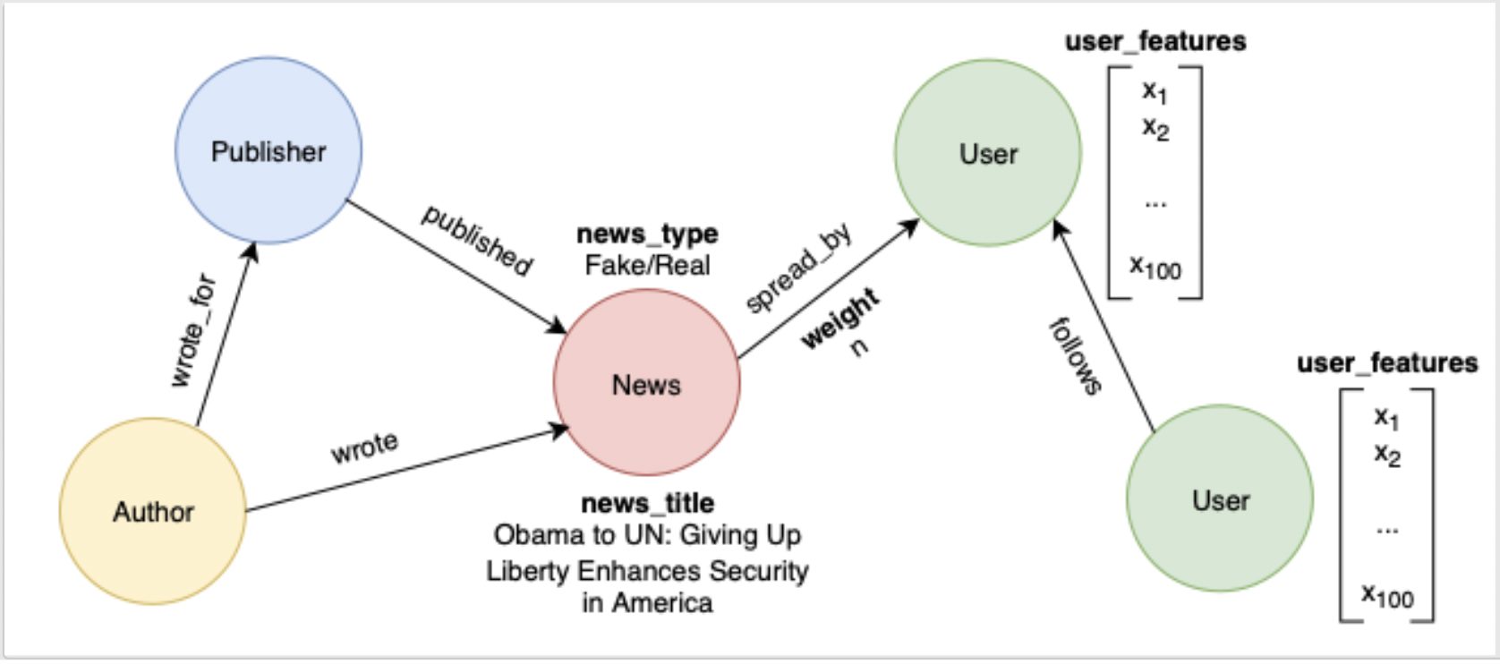
We processed the raw data from the FakeNewsNet repository and converted it into CSV format for vertices and edges in a heterogeneous property graph that can be readily loaded into a Neptune database with Apache TinkerPop Gremlin. The constructed property graph is composed of four vertex types and five edge types, as demonstrated in the following schematic, which together describe the social context in which each news item is published and shared. The News vertices have two properties: news_title and news_type (Fake or Real). The edges connecting News and User vertices have a weight property describing how many times the user has shared the news. The User vertices have a 100-dimension property representing user features such as age, gender, and historical social media activities (reduced from 109,626 to 100 using principal coordinate analysis).
The following screenshot shows the first 10 rows of the processed nodes.csv file.
The following screenshot shows the first 10 rows of the processed edges.csv file.
To follow along with this post, start by using the following AWS CloudFormation quick-start template to quickly spin up an associated Neptune cluster and AWS graph notebook, and set up all the configurations needed to work with Neptune ML in a graph notebook. You then need to download and save the sample dataset in the default Amazon Simple Storage Service (Amazon S3) bucket associated with your SageMaker session, or in an S3 bucket of your choice. For rapid experimentation and initial data exploration, you can save a copy of the dataset under the home directory of the local volume attached to your SageMaker notebook instance, and follow the create_graph_dataset.ipynb Jupyter notebook. After you generate the processed nodes and edges files, you can run the following commands to upload the transformed graph data to Amazon S3:
You can use the %load magic command, which is available as part of the AWS graph notebook, to bulk load data to Neptune:
You can use the %graph_notebook_config magic command to see information about the Neptune cluster associated with your graph notebook. You can also use the %status magic command to see the status of your Neptune cluster, as shown in the following screenshot.
Solution overview
Neptune ML uses graph neural network technology to automatically create, train, and deploy ML models on your graph data. Neptune ML supports common graph prediction tasks, such as node classification and regression, edge classification and regression, and link prediction. In our solution, we use node classification to classify news nodes according to the news_type property.
The following diagram illustrates the high-level process flow to develop the best model for fake news detection.
Graph ML with Neptune ML involves five main steps:
Export and configure the data – The data export step uses the Neptune-Export service to export data from Neptune into Amazon S3 in CSV format. A configuration file named training-data-configuration.json is automatically generated, which specifies how the exported data can be loaded into a trainable graph.
Preprocess the data – The exported dataset is preprocessed using standard techniques to prepare it for model training. Feature normalization can be performed for numeric data, and text features can be encoded using word2vec. At the end of this step, a DGL graph is generated from the exported dataset for the model training step. This step is implemented using a SageMaker processing job, and the resulting data is stored in an Amazon S3 location that you have specified.
Train the model – This step trains the ML model that will be used for predictions. Model training is done in two stages:
The first stage uses a SageMaker processing job to generate a model training strategy configuration set that specifies what type of model and model hyperparameter ranges are used for the model training.
The second stage uses a SageMaker model tuning job to try different hyperparameter configurations and select the training job that produced the best-performing model. The tuning job runs a pre-specified number of model training job trials on the processed data. At the end of this stage, the trained model parameters of the best training job are used to generate model artifacts for inference.
Create an inference endpoint in SageMaker – The inference endpoint is a SageMaker endpoint instance that is launched with the model artifacts produced by the best training job. The endpoint is able to accept incoming requests from the graph database and return the model predictions for inputs in the requests.
Query the ML model using Gremlin – You can use extensions to the Gremlin query language to query predictions from the inference endpoint.
Before we proceed with the first step of machine learning, let’s verify that the graph dataset is loaded in the Neptune cluster. Run the following Gremlin traversal to see the count of nodes by label:
If nodes are loaded correctly, the output is as follows:
126 author nodes
182 news nodes
28 publisher nodes
15,257 user nodes
Use the following code to see the count edges by label:
If edges are loaded correctly, the output is as follows:
634,750 follows edges
174 published edges
250 wrote edges
250 wrote_for edges
Now let’s go through the ML development process in detail.
Export and configure the data
The export process is triggered by calling to the Neptune-Export service endpoint. This call contains a configuration object that specifies the type of ML model to build, in our case node classification, as well as any feature configurations required.
The configuration options provided to the Neptune-Export service are broken into two main sections: selecting the target and configuring features. Here we want to classify news nodes according to the news_type property.
The second section of the configuration, configuring features, is where we specify details about the types of data stored in our graph and how the ML model should interpret that data. When data is exported from Neptune, all properties of all nodes are included. Each property is treated as a separate feature for the ML model. Neptune ML does its best to infer the correct type of feature for a property, but in many cases, the accuracy of the model can be improved by specifying information about the property used for a feature. We use word2vec to encode the news_title property of news nodes, and the numerical type for user_features property of user nodes. See the following code:
Start the export process by running the following command:
Preprocess the data
When the export job is complete, we’re ready to train our ML model. There are three machine learning steps in Neptune ML. The first step (data processing) processes the exported graph dataset using standard feature preprocessing techniques to prepare it for use by the DGL. This step performs functions such as feature normalization for numeric data and encoding text features using word2vec. At the conclusion of this step, the dataset is formatted for model training. This step is implemented using a SageMaker processing job, and data artifacts are stored in a pre-specified Amazon S3 location when the job is complete. Run the following code to create the data processing configuration and begin the processing job:
Train the model
Now that you have the data processed in the desired format, this step trains the ML model that is used for predictions. The model training is done in two stages. The first stage uses a SageMaker processing job to generate a model training strategy. A model training strategy is a configuration set that specifies what type of model and model hyperparameter ranges are used for the model training. After the first stage is complete, the SageMaker processing job launches a SageMaker hyperparameter tuning job. The hyperparameter tuning job runs a pre-specified number of model training job trials on the processed data, and stores the model artifacts generated by the training in the output Amazon S3 location. When all the training jobs are complete, the hyperparameter tuning job also notes the training job that produced the best performing model.
We use the following training parameters:
The hyperparameter tuning finds the best version of a model by running many training jobs on the dataset. You can summarize hyperparameters of the five best training jobs and their respective model performance as follows:
We can see that the best performing training job achieved an accuracy of approximately 94%. This training job will be automatically selected by Neptune ML for creating an endpoint in the next step.
Create an endpoint
The final step of machine learning is to create an inference endpoint, which is a SageMaker endpoint instance that is launched with the model artifacts produced by the best training job. We use this endpoint in our graph queries to return the model predictions for the inputs in the request. After the endpoint is created, it stays active until it’s manually deleted. Create the endpoint with the following code:
Our new endpoint is now up and running.
Query the ML model
Now let’s query your trained graph to see how the model predicts news_type for one unseen news node:
If your graph is continuously changing, you may need to update ML predictions frequently using the newest data. Although you can do this simply by rerunning the earlier steps (from data export and configuration to creating your inference endpoint), Neptune ML supports simpler ways to update your ML predictions using new data. See Workflows for handling evolving graph data for more details.
Conclusion
In this post, we showed how Neptune ML and GNNs can help detect social media fake news using node classification on graph data by combining information from the complex interaction patterns in the graph. For instructions on implementing this solution, see the GitHub repo. You can also clone and extend this solution with additional data sources for model retraining and tuning. We encourage you to reach out and discuss your use cases with the authors via your AWS account manager.
Additional references
For more information related to Neptune ML and detecting fake news in social media, see the following resources:
Beyond News Contents: The Role of Social Context for Fake News Detection
FakeNewsNet
Graph-based recommendation system with Neptune ML: An illustration on social network link prediction challenges
Analyzing social media feeds using Amazon Neptune
About the Authors
Hasan Shojaei is a Data Scientist with AWS Professional Services, where he helps customers across different industries such as sports, insurance, and financial services solve their business challenges through the use of big data, machine learning, and cloud technologies. Prior to this role, Hasan led multiple initiatives to develop novel physics-based and data-driven modeling techniques for top energy companies. Outside of work, Hasan is passionate about books, hiking, photography, and ancient history.
Sarita Joshi is a Senior Data Science Manager with the AWS Professional Services Intelligence team. Together with her team, Sarita plays a strategic role for our customers and partners by helping them achieve their business outcomes through machine learning and artificial intelligence solutions at scale. She has several years of experience as a consultant advising clients across many industries and technical domains, including AI, ML, analytics, and SAP. She holds a master’s degree in Computer Science, Specialty Data Science from Northeastern University.
Read MoreAWS Machine Learning Blog