According to a recent study, defective products cost industries over $2 billion from 2012–2017. Defect detection within manufacturing is an important business use case, especially in high-value product industries like the automotive industry. This allows for early diagnosis of anomalies to improve production line efficacy and product quality, and saves capital costs. Although advanced anomaly detection systems employ sensors as well as Internet of Things (IoT) devices to collect multimodal data to improve performance, computer vision continues to be a common approach. Detecting anomalies in automotive parts and components using computer vision can be done using normal images, and even X-Ray based images for structural damages. Recent advances in deep learning and computer vision have allowed scientists and manufacturers to develop enhanced anomaly detection systems, including surface defect detection on automotive body panels and dent detection in vehicles.
Anomaly detection typically consists of two tasks: detecting whether a given product is defective or not, and localization of the defect—the process of identifying the exact location of a defect inside of an image. In this post, we show how we designed and implemented an end-to-end pipeline for the following:
Defect detection using Amazon Lookout for Vision, a machine learning (ML) service for identifying anomalies in images using computer vision
Defect localization through supervised and unsupervised approaches using Amazon SageMaker
The supervised approach based on Single Shot MultiBox Detector (SSD) is relevant in use cases where we have sufficient labeled data. However, creating annotations for images can often be expensive and time-consuming. Additionally, anomalous images aren’t usually available at a high scale by definition. For these use cases, we present an unsupervised defect localization method based on a variational autoencoder (VAE).
Data overview
In the automotive space, the most common types of defects shown in the following table can be categorized into the following:
Dimensional – Such as orientation, alignment, and roundness
Structural – Such as holes, screws, and clamps
Surface – Such as scratches, cracks, wear, and roughness
Operational defects – Incompatibility to standards and specifications
In this post, we worked with automotive parts such as wheels and knuckles.
Defects
Types
Details
Dimensional
Dimensions, Shape, Positioning, Orientation, Alignment, Roundness, Corners
Structural
Assembly, Holes, Slots, Rivets, Screws, Clamps
Foreign Objects, Dust, Bur, Swarm
Surface
Pits, Scratches, Cracks, Wear, Finish, Roughness, Texture, Seams-Folds-Laps, Continuity
Operational
Incompatibility of Operation to Standards and Specifications
We utilized the GRIMA X-Ray database GDXray dataset, which includes five groups of images: casting, welding, baggage, nature, and settings (see the following table).
Group
Classes
Images
Casting
67
2,727
Welds
3
88
Baggage
77
8,150
Nature
13
8,290
Settings
7
152
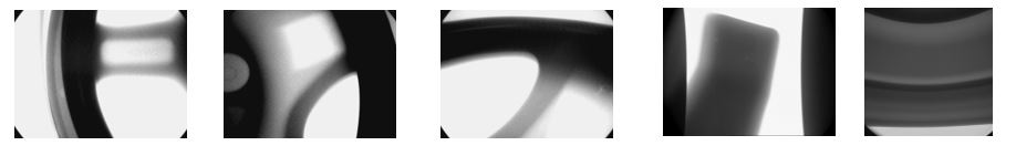
We considered the castings data for this project, which included 2,727 X-Ray images. We excluded four images due to them not resembling wheels or knuckles, leaving us with 984 defective and 1739 non-defective. The following images show some examples from the dataset used in this study.
We used different sample sizes for training and testing due to different requirements for the underlying modeling approaches. The following table displays the number of samples used in each of our models for training and testing.
Model
Training
Testing
Lookout for Vision (classification)
2179
544
Custom Variational Autoencoder (unsupervised)
1739
984
Custom Single Shot Multibox Detector (supervised)
544
1036
Defect detection using Lookout for Vision
Lookout for Vision is an ML service that spots defects and anomalies in visual representations using computer vision. With Lookout for Vision, manufacturing companies can increase quality and reduce operational costs by quickly identifying differences in images of objects at scale. For example, you can use Lookout for Vision to identify missing components in products, damage to vehicles or structures, irregularities in production lines, miniscule defects in silicon wafers, and other similar problems.
Lookout for Vision uses ML to see and understand images from any camera as a person would, but with an even higher degree of accuracy and at a much larger scale. Lookout for Vision allows you to eliminate the need for costly and inconsistent manual inspection while improving quality control, defect and damage assessment, and compliance. In minutes, you can begin using Lookout for Vision to automate inspection of images and objects with no ML expertise required. Using Lookout for Vision to classify images as anomalous (defective) or non-defective is a crucial step in our pipeline for identifying which images need further analysis.
Lookout for Vision process and results
We completed the process of model development using Lookout for Vision in three steps:
We uploaded our sample data to Amazon Simple Storage Service (Amazon S3) into training and testing folders, and we linked them to our Lookout for Vision project.
We trained our classification model through the Lookout for Vision user interface using the uploaded dataset.
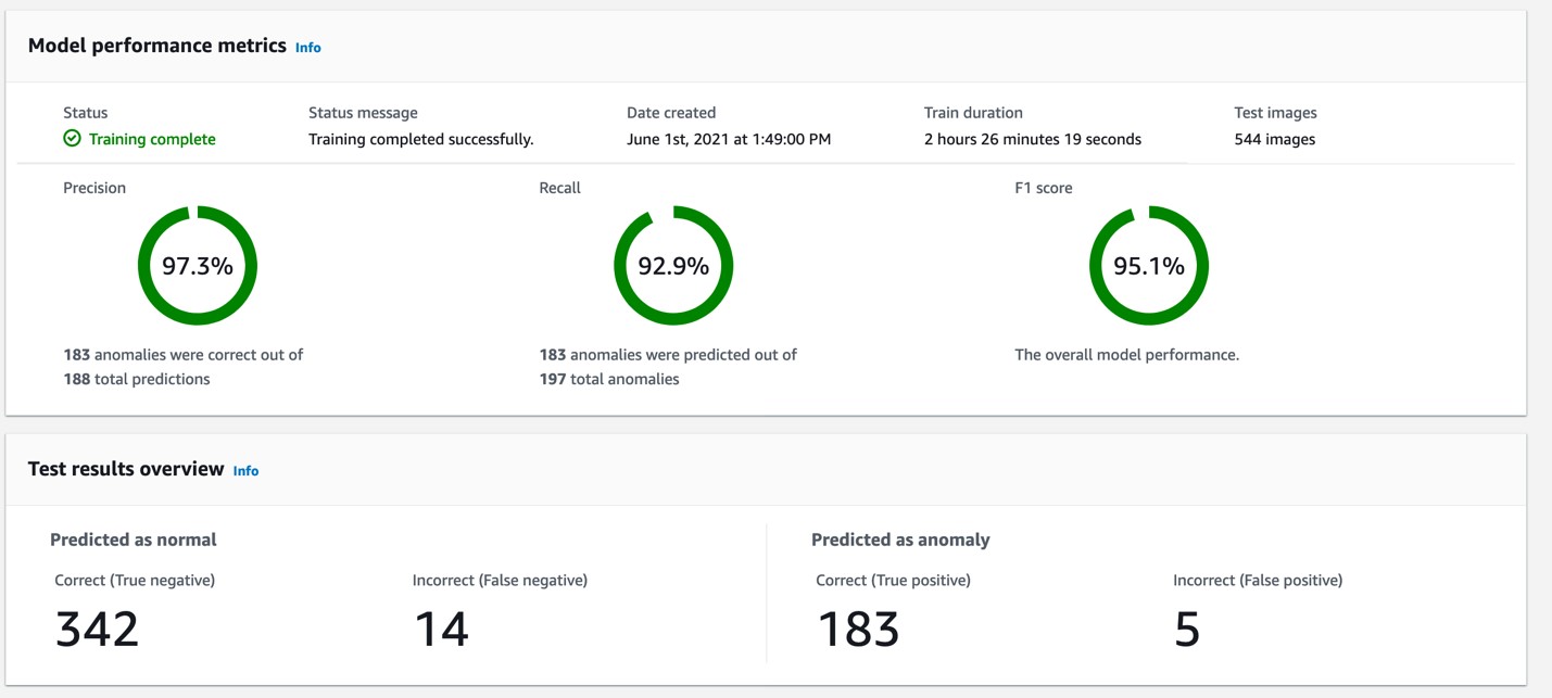
When the training was complete, we analyzed the results for the testing set, illustrated in the following figure.
Lookout for Vision enabled us to detect defective images in our dataset and prepare our samples for localizing defective regions in the shortlisted dataset. Lookout for Vision helped identify 183 anomalous images correctly, out of which 123 samples were used for training of the defect localization model. The remaining 60 samples were used for testing. The localization pipeline and results from our approach are described in the following section. Using a system such as Lookout for Vision, which facilitates the identification of defective parts, followed by our defect localization pipeline described in the next section, facilitates an end-to-end defect detection pipeline.
Defect localization pipeline
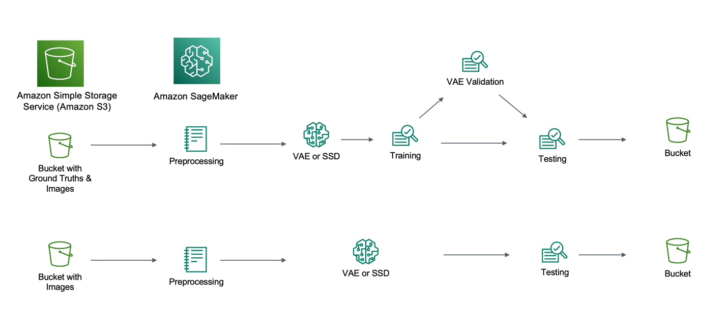
Defect localization is the process of identifying the exact location of a defect inside of an image. We developed a defect localization pipeline with two options. The first option allows you to provide your data to train ML models. We describe two approaches for training, one using an unsupervised VAE, and another using a supervised SSD method. The second option allows you to use only pretrained or custom models for prediction purposes without training. The following figure illustrates the details of the pipeline developed in this work.
In the first option, we upload the data into an S3 bucket separated into defective and non-defective folders, which are fed into the processing pipeline. The following is a snippet of the VAE training process:
net = VAE(n_hidden=n_hidden, n_latent=n_latent, n_layers=n_layers, n_output=n_output, batch_size=1)
net.collect_params().initialize(mx.init.Xavier(), ctx=model_ctx)
net.hybridize()
trainer = gluon.Trainer(net.collect_params(), ‘adam’, {‘learning_rate’: .00001})
# Training VAE MODEL
n_epoch = 40
print_period = n_epoch // 10
start = time.time()
training_loss = []
validation_loss = []
for epoch in tqdm(range(n_epoch)):
epoch_loss = 0
epoch_val_loss = 0
train_iter.reset()
test_iter.reset()
n_batch_train = 0
for batch in train_iter:
n_batch_train +=1
data = batch.data[0].as_in_context(model_ctx)
data = data.reshape(train_iter.batch_size, 768**2)*(1/255)
with autograd.record()
loss = net(data)
loss.backward()
trainer.step(data.shape[0])
epoch_loss += nd.mean(loss).asscalar()
n_batch_val = 0
for batch in test_iter:
n_batch_val +=1
data = batch.data[0].as_in_context(model_ctx)
data = data.reshape(train_iter.batch_size, 768**2)*(1/255)
loss = net(data)
epoch_val_loss += nd.mean(loss).asscalar()
epoch_loss /= n_batch_train
epoch_val_loss /= n_batch_val
training_loss.append(epoch_loss)
validation_loss.append(epoch_val_loss)
if epoch % max(print_period,1) == 0:
tqdm.write(‘Epoch{}, Training loss {:.2f}, Validation loss {:.2f}’.format(epoch, epoch_loss, epoch_val_loss))
end = time.time()
print(‘Time elapsed: {:.2f}s’.format(end – start))
net.save_parameters(model_prefix)
After preprocessing, we fed all the non-defective images into the model. The following code is the training process for SSD:
net = get_model(‘ssd_512_mobilenet1.0_coco’, pretrained=True, ctx=ctx)#ssd_512_mobilenet1.0_coco
net.reset_class(classes)
train_data = get_dataloader(net, dataset, 512, 1, 0, ctx)
net.collect_params().reset_ctx(ctx)
trainer = gluon.Trainer(
net.collect_params(), ‘sgd’,
{‘learning_rate’: 0.0001, ‘wd’: 0.0005, ‘momentum’: 0.9})
mbox_loss = gcv.loss.SSDMultiBoxLoss()
ce_metric = mx.metric.Loss(‘CrossEntropy’)
smoothl1_metric = mx.metric.Loss(‘SmoothL1’)
print(“Starting SSD Training”)
for epoch in range(40):
ce_metric.reset()
smoothl1_metric.reset()
tic = time.time()
btic = time.time()
net.hybridize(static_alloc=True, static_shape=True)
for i, batch in enumerate(train_data):
batch_size = batch[0].shape[0]
data = gluon.utils.split_and_load(batch[0], ctx_list=[ctx], batch_axis=0)
cls_targets = gluon.utils.split_and_load(batch[1], ctx_list=[ctx], batch_axis=0)
box_targets = gluon.utils.split_and_load(batch[2], ctx_list=[ctx], batch_axis=0)
with autograd.record():
cls_preds = []
box_preds = []
for x in data:
cls_pred, box_pred, _ = net(x)
cls_preds.append(cls_pred)
box_preds.append(box_pred)
sum_loss, cls_loss, box_loss = mbox_loss(
cls_preds, box_preds, cls_targets, box_targets)
autograd.backward(sum_loss)
# since we have already normalized the loss, we don’t want to normalize
# by batch-size anymore
trainer.step(1)
ce_metric.update(0, [l * batch_size for l in cls_loss])
smoothl1_metric.update(0, [l * batch_size for l in box_loss])
name1, loss1 = ce_metric.get()
name2, loss2 = smoothl1_metric.get()
if i % 100 == 0:
print(‘[Epoch {}][Batch {}], Speed: {:.3f} samples/sec, {}={:.3f}, {}={:.3f}’.format(
epoch, i, batch_size/(time.time()-btic), name1, loss1, name2, loss2))
btic = time.time()
net.save_parameters(ssd_model_name)
The preceding snippet was taken from GluonCV.
In the second option, data is uploaded into an S3 bucket in a single folder. The images are fed into the pipeline, and an already built model (pretrained or custom) is called to make the prediction. Predictions are uploaded back to the same bucket.
Unsupervised defect localization
For the first model in the localization pipeline, we employed a VAE as the unsupervised method, in which we employed data without labels. For testing, we selected an image at random and fed it into the autoencoder, with the expectation that the reconstructed image would be a replica of the original, except for the defect (if present). The entire process is as follows:
We passed images through the autoencoder to generate feature maps.
We reconstructed the generated feature maps using a L2 normalization transformation.
This L2 image is then multiplied with the original to have higher contrast in the areas where defects are present.
We used the final version of the image to create a binary mask where anomalous pixels are labeled as 1 and 0, otherwise using an optimal threshold on the pixel intensity based on validation data.
After we created the binary mask, we removed the false positives using only “largely” connected pixels, and we generated the bounding boxes using the remaining pixels.
The following figure demonstrates the VAE architecture.
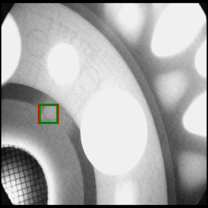
The following image is an example of a predicted bounding box (red) by VAE and ground truth (green).
Supervised defect localization
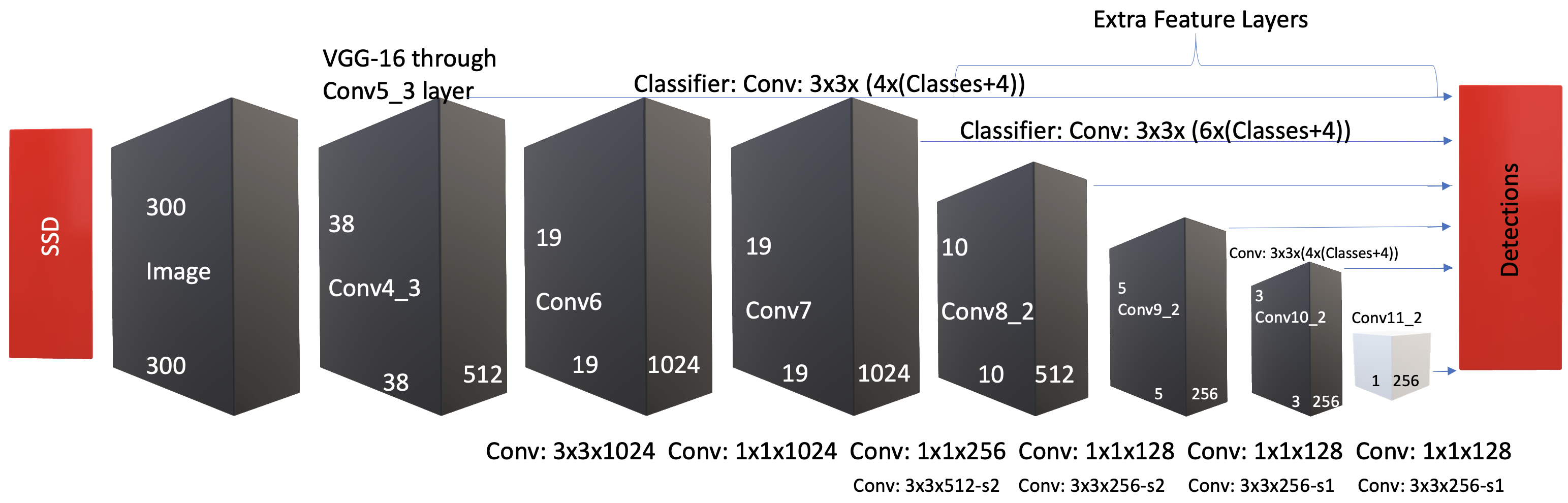
The second model of the localization pipeline, the supervised approach, uses the SSD algorithm with a MobileNet backbone in place of VGG-16 pretrained on the Common Objects in Context (COCO) dataset. We followed a similar pipeline structure as the unsupervised VAE method for testing. We randomly selected images from our data and fed them into the network. The network output the coordinates for bounding box predictions of the defects. Then, we uploaded all of the images to the original S3 bucket with all the detected defects surrounded by bounding boxes. The original SSD architecture is depicted in the following figure.
The following image is an example of a predicted bounding box (red) by SSD and ground truth (green).
To evaluate our methods, we used the F1 score and intersection over union (IoU). The results are shown in the following table. In the baseline model, an F1 score of 19% and an IoU of 10% were produced by the VAE method. We could significantly increase the F1 score to 46% and our IoU to 26% with our object detection model pretrained on COCO.
Method
Training Split
Testing Split
Avg F1
Avg IOU
Best F1
Best IOU
VAE
1739
984
19%
10%
88%
80%
SSD
544
1036
46%
26%
96%
89%
Lookout for Vision
2179
544
95.1%
–
–
–
Summary
We implemented a deep learning-based solution for defect detection and localization in automotive parts based on supervised and unsupervised methods. After you have detected all the anomalous (defective) images using Lookout for Vision, you can apply our defect localization pipeline to localize defective regions in anomalous images. Our solution, developed using SageMaker, allows you to upload data into an S3 bucket and run the commands via the terminal to train the models or predict defects in unseen data. The unsupervised VAE model enables customers without labeled data to localize defects, whereas the supervised object detection method requires labeled data, resulting in more accurate defect localization.
Use your manufacturing images in our pipeline to reduce defects and improve the efficiency of your assembly line. Visit our website to learn more about the Amazon ML Solutions Lab and what it can do for your organization!
About the Authors
Matthew Rhodes is a Data Scientist in the Amazon ML Solutions Lab here at AWS. He has experience in computer vision and natural language processing, and graduated from Michigan State University with a B.S. in computer science. He went on to University of Washington where he graduated with a Master’s in Data Science.
Saman Sarraf is a Senior Applied Scientist at the Amazon ML Solutions Lab. His background is in applied machine learning including deep learning, computer vision, and time series data prediction.
Suchitra Sathyanarayana is a Senior Manager, Applied Science at the Amazon ML Solutions Lab where she helps AWS customers across different industry verticals accelerate their AI and cloud adoption. She holds a PhD in Computer Vision from Nanyang Technological University, Singapore.
Read MoreAWS Machine Learning Blog

