

Online bookmakers are innovating to offer their clients continuously updated sports data feeds that allow betting throughout the duration of matches. In this post, we walk through a solution to ingest, store, and stream sports data feeds in near real-time using Amazon API Gateway, Amazon DynamoDB, and Amazon Kinesis Data Streams.
In betting, odds represent the ratio between the amounts staked by parties to a bet. The odds for a given outcome of a sporting match change in response to events within the match. Sports data providers supply a variety of data feeds, such as game details and odds. Online bookmakers consume these data feeds to publish to their sports trading analysts. As odds change based on the events in the game, sports trading analysts use the continuously updated information from the data feeds to manage bets and odds. In order to remain competitive, bookmakers must provide updated odds to trading analysts in near-real time.
The solution presented in this post provides near real-time streaming of sports data feeds to a front-end application, allowing sports trading analysts to make decisions for online bookmakers based on the latest sports data feeds.
Solution overview
The solution uses serverless services—which offload the undifferentiated heavy lifting aspects of infrastructure and maintenance to Amazon Web Services (AWS)—allowing you to focus on the application logic. Our solution has the following components:
Sports data provider – External entities that provide on-field and off-field sports data feeds.
Backend database (DynamoDB) – The sports data feeds are stored in a DynamoDB table to support historical queries for charting and data retention purpose.
Application layer – AWS Lambda functions handle the application logic and reading and writing data into the DynamoDB table.
Front-end application – Renders the continuously changing sports data feeds for monitoring and analysis purposes.
API layer – Integrates the front-end application and sport data provider with the backend application. API Gateway provides an API layer for ingesting the data feeds from sports data providers using REST APIs.
Change data capture – To identify the continuously changing sports data feeds and stream to the front-end application. The changes to the sports data feeds are captured from Kinesis Data Streams for DynamoDB using a Lambda function and then published via WebSocket APIs to the front-end application.
WebSocket connection – Persistent connection from the front-end application to the API and backend application. API Gateway WebSocket APIs are used to achieve persistent connections to publish and display the continuously changing sports data feeds.
Sports trading analyst – The primary users of the solution that will be monitoring and analysing the sports data feeds using the front-end application.
Data flow
The data flow in the solution can be divided into two flows:
Flow A: Sports data provider to DynamoDB
The sports data provider continuously posts the sports data feeds.
API Gateway serves as a data ingestion layer for the sports data feeds.
Lambda functions implement the application logic to write the sports data feeds.
DynamoDB handles the persistent storage of the sports data feeds.
Flow B: DynamoDB to front-end application
Kinesis Data Streams captures the change records from the DynamoDB table when new feeds are inserted.
The StreamConsumer Lambda function receives the change event record from the stream.
The odds feed data is published to the front-end application via WebSocket connections.
The sports trading analyst monitors and analyse the sports data feeds from the front-end application.
Figure 1 illustrates the solution architecture and the two flows described above.
Next, we work through in detail how the sports data feeds are ingested, stored, and streamed to the front-end application.
Data ingestion
API Gateway REST API handles the data ingestion.
Sports data providers support various options for consuming the data feeds. For this use case, we assume that the sports data provider posts a continuous stream of odds data feeds. The following is a sample odds data feed for a game:
“summary”:”UEFA European Championship @ Wembley”,
“gameId”:”ftge2gq-4g6daf1″,
“gameDate”:”2021-11-20 16:00″,
“isOpen”:true,
“away”:3,
“home”:-3,
“awayOdds”:-110,
“homeOdds”:-110,
“date”:”2021-11-20 20:30:15.238″
}
You might need to source these data feeds from multiple sports data providers. Features like API Gateway usage plans and API keys can help with rate-limiting and identifying the data sources. The REST API in API Gateway is subscribed with the sports data providers to post the data feeds.
The ingestion of data feeds is handled by the API Gateway REST API resource named /feeds with the PUT method configured to use the backend integration type as LAMBDA_PROXY, which is associated with the Lambda function WriteFeeds. Likewise, to read data feeds, the GET method of the API Gateway REST API resource /feeds is configured to use the backend integration type as LAMBDA_PROXY, which is associated with the Lambda function ReadFeeds. The GET method of the feeds API can be used by the front-end application for querying the feeds needed for the initial rendering. For more information, see Creating a REST API in Amazon API.
Figure 2 shows the PUT method configuration of the /feeds REST API associated with the WriteFeeds Lambda function. The GET method has the same configuration but is associated with ReadFeeds Lambda function.
Data store
To handle storage for our use case, we use the following resources:
A DynamoDB table for persistent storage
NoSQL Workbench for data modeling
The WriteFeeds Lambda function
DynamoDB stores the sports data feeds. DynamoDB is serverless, which means we can offload the heavy lifting maintenance, patching, and administration of the infrastructure to AWS. With a NoSQL database service such as DynamoDB, data modeling is different than modeling with a relational database. In relational data modeling, we start with entities first. With a normalized relational model, we can create any query pattern needed in your application. But NoSQL databases are designed for speed and scale. Although the performance of the relational database might degrade as you scale up, horizontally scaling databases such as DynamoDB provide consistent performance at any scale.
With DynamoDB, you design your schema specifically to make the most common and important queries as fast and as inexpensive as possible. After identifying the required access patterns, you can organize data by keeping related data in close proximity for the benefit of cost and performance. As a general rule, you should maintain as few tables as possible and preferably start with a single table so that all related items are kept as close together as possible. You can use the NoSQL Workbench to help visualize your queries and create the DynamoDB resources. NoSQL Workbench is a unified visual IDE tool that provides data modeling, data visualization, and query development features to help you design, create, query, and manage DynamoDB tables.
Data model
The first step in data modeling is to identify all the entities in the application and how they relate to each other, as shown in Figure 3. In this use case, we have the following entities:
Game – The name of the games
Odds – The odds feed for a game
Client – The trading analyst connected to the application displaying the odds feeds
Connection – Web Socket connection from the client
The game entity represents the game ID, name, type, venue, status, and team details of different games. For example, game-cricket can be used as the type to identify a game and game-soccer can be the type for the soccer game. Feeds represent the actual data for the game odds provided by the sports data provider. The odds data feed is composed of a timestamp, game ID and several other fields with data values. Clients in this use case represent the trading analysts logged in to the application and consume the odds feeds in the form of charts, graphs, and tables. The connection entity holds the persistent WebSocket connections through which the odds data feeds are published in near real-time.
Access patterns
The next step with a NoSQL design is to identify all the required access patterns for the application prior to the schema design. It is important to ensure your data model matches your access patterns to optimize performance. In addition, capturing the frequency of invocation of these access patterns helps you determine the right capacity configurations for your tables. The following table shows an example of the different access patterns possible.
Access pattern
Frequency
Create a game
Less: approximately 100 per day
Insert odds feeds
High during multiple games: approximately 500 per second
Insert client connection
Low and as trading analysts connect: approximately 10 per min
Lookup all scheduled games
Low: approximately 100 per hour
Lookup game details by game id
Low: approximately 100 per hour
Get latest odds feed for a given game id
Low: approximately 100 per hour
Get odds feeds for a date range sorted by odds timestamp
Low: approximately 100 per hour
Get all active client connections
High and invoked for every odds inserted: approximately 500 per second
Schema design
We use a single table design to model the NoSQL schema for all the entities identified in the data modeling step earlier. Using a single table reduces the need to make multiple requests, which is very important in terms of latency for real-time applications. We use generic attributes, PK and SK, for the partition key and sort key so that we can overload it for all the identified entities. For each game entity, we use its name as the partition key. The sort key is made up of an identifier game and the type of the game (game-cricket or game-soccer). This helps identify and group the different games based on the game types. For more information about choosing the right partition key when designing the schema for DynamoDB, read Choosing the Right DynamoDB Partition Key.
NoSQL Workbench is useful, particularly during the early stages of development for visualizing the data model and when you experiment and make changes regularly as you progress with the design. After you finalize the schema, the recommendation is to adopt an infrastructure as code approach by using AWS CloudFormation, AWS Cloud Development Kit (AWS CDK), or AWS Serverless Application Model (AWS SAM).
Figure 4 shows the aggregate view from the NoSQL Workbench visualizer of the data model with sample table values.
In addition to the primary key, applications might need one or more secondary keys to allow efficient access to data and to support different query patterns. DynamoDB allows you to create one or more secondary indexes on a table and issue query or scan requests against these indexes. Secondary index contains a subset of attributes from a table, along with an alternate key to support query operations. DynamoDB supports two types of secondary indexes.
Global Secondary Indexes (GSI) – An index with a partition key and sort key that can be different from those on the base table.
Local secondary Index (LSI) – An index that has the same partition key as the base table, but a different sort key.
When you create a GSI, you specify a partition key and optionally a sort key. Only items in the base table that contain those attributes appear in the index. GSIs are sparse by default. A sparse GSI can be used for access patterns where you need to query a subset of the items from the base table where an attribute is not present on all items.
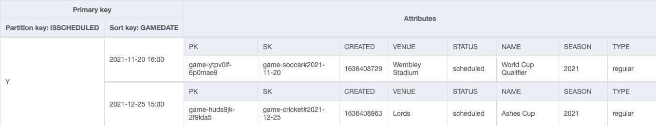
The partition key and sort key of the table isn’t always sufficient to accomplish all the different query access patterns. You can opt for creating a GSI for those access patterns that need a different attribute as the partition key. For the access pattern to look up all the scheduled games, we create an index (GSI-1) and use the sparse GSI pattern with the ISSCHEDULED attribute as the partition key of the GSI and GAMEDATE as the sort key. This means only the items that have the attribute ISSCHEDULED are available in the index, reducing the number of items that can be separately queried in the index. The sort key can also support sorting and paginating the results in the UI. Figure 5 shows GSI-1 being used to look up all scheduled games.
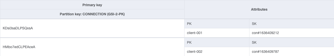
To retrieve all active connections, we create another sparse index (GSI-2) using the CONNECTION attribute as the partition key of the index. We can’t scan the entire table with millions of odds data, so a sparse GSI enables us to retrieve all the connections using a scan operation against the index with the subset of the items from the base table. Figure 6 shows GSI-2 being used to retrieve all active connections.
Next, we included an EXPIRE attribute for the items that we plan to delete using the DynamoDB TTL settings. This is useful for items like WebSocket connections where there are possibilities of stale connections. We can enforce a TTL expiration time to delete these connections after a certain duration. The odds feed data items can grow voluminous depending on how often you choose to receive data from the sports data providers, therefore we can use the TTL expiration for the odds feed data items as well. You might need to store these odds data items for charting and graph needs, but you can set the expiration time to match how long you want to retain the feed, such as 6 months or 1 year.
The following table summarizes the read access patterns and their query conditions.
Access pattern
Query conditions
Look up all scheduled games
Use GSI-1, scan the sparse GSI
Look up game details by game id
Primary key on table, PK = game-ytpv0if-6p0mae9
Get latest odds feed for a game
Primary key on table, PK= game-ytpv0if-6p0mae9, SK begins-with odds-, scanIndexForward=false, Limit=1
Get all odds for a date range of a game
Primary key on table, PK= game-ytpv0if-6p0mae9, SK BETWEEN odds-Date
Get all active WebSocket connections
Use GSI-2, scan the sparse GSI
WriteFeeds Lambda function
Now that we have created the DynamoDB table, we can look at the Lambda function WriteFeeds, which handles writing the odds feed data received through the API Gateway REST API resource /feeds. To test the application, we use a simulated sports data provider script that sends odds feeds for about 10 games together in a single PUT request. The WriteFeeds function uses the ddb.batchWriteItem() API method to batch all 10 writes together in a single request. By combining multiple writes in a single request, BatchWriteItem allows us to achieve parallelism without having to manage it at the application level. We generally use BatchWriteItem when dealing with large amounts of data and also for the use cases where the programming language used has no easier mechanisms for multi-threading and parallelism.
The following WriteFeeds Lambda function demonstrates using the BatchWriteItem API for storing the ingested odds feeds into the DynamoDB table:
AWS.config.region = process.env.REGION
const tableName = process.env.TABLE_NAME
const ddb = new AWS.DynamoDB({ apiVersion: “2012-08-10” })
exports.handler = async (event) => {
console.log(“Received event:”, JSON.stringify(event, null, 2))
let odds = JSON.parse(event.body).odds
let requestsArray = []
//to write feeds to sportsfeeds table
for (let i = 0; i < odds.length; i++) {
let created = String(Math.floor(new Date().getTime() / 1000))
//epoch timestamp for TTL attribute to automatically delete items after 1 year
let expire = String(
Math.floor(
new Date(new Date().setFullYear(new Date().getFullYear() + 1)) / 1000
)
);
requestsArray.push({
PutRequest: {
Item: {
PK: { S: odds[i].gameId },
SK: { S: “odds-” + odds[i].date},
AWAY: { N: odds[i].away.toString() },
HOME: { N: odds[i].home.toString() },
AWAYODDS: { N: odds[i].awayOdds.toString() },
HOMEODDS: { N: odds[i].homeOdds.toString() },
CREATED: { N: created },
EXPIRE: { N: expire }
},
},
})
}
let params = {
RequestItems: {
[tableName]: requestsArray,
}
}
console.log(“Batch Write of Feeds – begin.”)
try {
const data = await ddb.batchWriteItem(params).promise()
console.log(“Batch Write of Feeds – end”)
} catch (err) {
console.log(“Error adding Batch Items :” + err)
}
const response = {
statusCode: 200,
body: JSON.stringify(“Feeds Added Successfully”),
}
return response
}
Data stream
The data stream aspect of the use case is handled by the following resources:
A DynamoDB table with streams enabled
Kinesis Data Streams
The StreamConsumer Lambda function
The API Gateway Management API
There are several factors to consider when choosing the right streaming solution; we discuss in this section how we evaluated these factors for our use case.
First, DynamoDB offers two options for streaming the change data capture (CDC): Kinesis Data Streams for DynamoDB and DynamoDB Streams. We referred to Streaming Options for Change Data Capture to choose Kinesis Data Streams as the streaming model for this application’s latency requirements. The number of shards and consumers per shard are an important aspect of streaming. With Kinesis Data Streams, we can read with a maximum of five consumer processes per shard or up to 20 simultaneous consumers per shard with enhanced fan-out, versus two per shard for DynamoDB Streams.
The second factor is to decide between using a shared throughput consumer or a dedicated throughput consumer with Kinesis Data Streams. The dedicated throughput with enhanced fan-out gets a dedicated connection to each shard, and is used when you have many applications read the same data, or if you’re reprocessing a stream with large records. In our use case, we needed low latency and high throughput, so we chose the dedicated throughput consumer with enhanced fan-out.
The third factor is to decide how to read from the data stream with the options like Lambda, Kinesis Data Analytics, Kinesis Data Firehose, and the Kinesis Client Library (KCL). The KCL requires a custom-built consumer application instance, and also requires worker instances to process the data. Data Firehose is a more appropriate choice when you want to deliver real-time streaming data to destinations such as Amazon Simple Storage Service (Amazon S3), Amazon Redshift, Amazon OpenSearch Service (successor to Amazon Elasticsearch Service), and Splunk. For analyzing and enriching the data, a Data Analytics application is another choice. You can use Lambda functions to automatically read and process batches of records off your Kinesis stream. Lambda periodically polls the Kinesis stream for new records (70-millicecond latency). When Lambda detects new records, it invokes the StreamConsumer Lambda function, passing the new records as parameters.
From all the options listed, we decided to use Lambda because it natively integrates with Kinesis Data Streams, abstracting the polling, check pointing, and error handling complexities, and allowing us to focus only on the data processing logic. Also, in our use case, the odds feed data is already normalized and ready to be sent as-is to the front-end application without any further enrichment.
The fourth factor is to decide on how many shards, because shards are the base throughput unit when using Kinesis Data Streams. You can use the following formula to decide on the number of shards needed to accommodate your DynamoDB streaming throughput:
For our use case, we estimated the initial number of shards needed with the calculation:
Average record size in DynamoDB table = 1000 bytes
Maximum number of write operations per second = 3000
Percentage of update and overwrite compared to create and delete = 0
You can use the Shard Estimator on the Kinesis Data Streams console, on the Capacity configuration page.
The next factor we considered is the tuning parameters related to Lambda and Kinesis Data Streams.
Lambda invokes the function as soon as records are available in the stream. To control invoking the function until there is a large enough batch of records, you can configure the batch window so that the Lambda function continues to gather records from the stream until it has gathered a full batch or until the batch window expires. For our use case, we couldn’t allow the function to wait beyond 1 second and so didn’t configure the batch window size.
The Lambda function might return an error when processing the received stream records. If that happens, the function tries to process the entire batch again, resulting in possible duplicates or even stalling the processing. During the development stage of the application, we frequently experienced these problems and the remedy was to reduce the maximum retry attempts and the maximum age of records that the function includes for processing. You can also enable the Split batch on error setting to overcome the issue. Another approach is to allow the function to always return success by handling exceptions in a catch block, logging them to Amazon Simple Queue Service (Amazon SQS) or Amazon CloudWatch Logs for further analysis and troubleshooting.
The following screenshot from the Lambda console shows the Lambda and Kinesis data stream integration, highlighting the important configuration properties, including batch window, retry attempts, maximum age of records, split batch on error.
StreamConsumer Lambda function
The StreamConsumer Lambda function has been mapped to the Kinesis data stream to receive the CDC records (odds feeds) from DynamoDB. Each odds-feed record corresponds to a change in the odds value of the associated game. The function finds all the active front-end client applications using their WebSocket connections persisted in the table. Using the API Gateway Management API and the WebSocket connection, the odds data is published to the front-end application.
The following code is the StreamConsumer Lambda function:
AWS.config.region = process.env.REGION
const tableName = process.env.TABLE_NAME
const docClient = new AWS.DynamoDB.DocumentClient()
const parse = AWS.DynamoDB.Converter.output
exports.handler = async (event) => {
var records = event.Records
console.log(“Recieved Event :” + JSON.stringify(event))
//to traverse kinesis stream records to process stream
const asyncRes = await Promise.all(
records.map(async (record) => {
var payload = Buffer.from(record.kinesis.data, “base64”).toString(
“ascii”
)
var jsonpayload = JSON.parse(payload)
if (jsonpayload.eventName == “INSERT”) {
var image = parse({ M: jsonpayload.dynamodb.NewImage })
console.log(image);
var feed = {
“gameId”: image.PK,
“away”: image.AWAY,
“home”: image.HOME,
“awayOdds”: image.AWAYODDS,
“homeOdds”: image.HOMEODDS,
“date”: image.CREATED
}
console.log( “feed :” + feed)
var connections = await findAllConnections()
var items = connections.Items
const asyncResp = await Promise.all(
items.map(async (item) => {
var conn = item.CONNECTION
var endpoint = item.ENDPOINT
await pushDataToClient(conn, endpoint, feed)
})
)
}
})
)
const response = {
statusCode: 200,
body: JSON.stringify(“StreamConsumer – Succeeded publishing”),
}
return response
}
// scan for connections in the sparse GSI-CON
async function findAllConnections() {
try {
var params = {
TableName: tableName,
IndexName: “GSI-CON”,
ProjectionExpression: “#PK, CLIENT, ENDPOINT”,
ExpressionAttributeNames: {
“#PK”: “CONNECTION”,
},
}
const connections = await docClient.scan(params).promise()
return connections
} catch (err) {
return err;
}
}
//to publish feeds to websocket connection
async function pushDataToClient(connectionId, endpointURL, feed) {
try {
const apigwManagementApi = new AWS.ApiGatewayManagementApi({
apiVersion: “2018-11-29”,
endpoint: endpointURL,
})
console.log(“pushToConnection : ” + connectionId + ” feed : ” + JSON.stringify(feed))
var testfeed=”Test feed”
var resp = await apigwManagementApi
.postToConnection({ ConnectionId: connectionId, Data: JSON.stringify(feed) })
.promise()
return resp;
} catch (err) {
return err;
}
}
Deploy and test the solution
AWS CDK is used to deploy the solution to an AWS account. The AWS CDK is an open-source software development framework that you can use to define cloud infrastructure in a familiar programming language and provision it through AWS CloudFormation.
The CDK deployment script creates the following resources:
API Gateway resources – feedsAPI (REST API) and bookmakerAPI (WebSocket API)
Lambda functions – writeFeeds, readFeeds, connectionManager, and streamConsumer
DynamoDB table – sportsfeeds
Kinesis data stream – feedstream
Prerequisites
You must have the following prerequisites in place in order to deploy and test this solution:
An AWS account.
The wscat utility installed for testing WebSocket APIs. For instructions, refer to Use wscat to connect to a WebSocket API and send messages to it.
Development terminal.
Node.js installed. For more information, see the Node.js website.
AWS CLI already installed.
AWS CDK already installed.
Clone the repository and deploy
The code for the solution in this post is located in the GitHub repository and can be cloned and run using the following commands:
Clone the repository to your local development machine:
Install AWS CDK and dependencies:
npm install -g aws-cdk
cdk –version
npm install –save-exact @aws-cdk/aws-lambda @aws-cdk/aws-lambda-nodejs @aws-cdk/aws-dynamodb @aws-cdk/aws-apigatewayv2 @aws-cdk/aws-kinesis @aws-cdk/aws-apigatewayv2-integrations @aws-cdk/aws-lambda-event-sources
Configure AWS access key and secret access key:
Bootstrap the AWS account:
Deploy all the AWS resources:
Test the solution
Now that the solution is deployed, the next step is to test its workflow.
Initialize with sample game data
The repository includes the initDB.sh script to initialize the table with some sample data for the games and client entities. Run the script using the command below:
sh initDB.sh
Start the front-end client application
To simulate the front-end client application, use the wscat tool to create a WebSocket client connection request. You can create multiple sessions from different terminals using the following example command on each terminal. You can get the bookmakerAPI URL from the API Gateway console.
Generate the odds feed
The repository provides a script to generate a sample odds feed for different games. You can get the feedsAPI URL from the API Gateway console. To generate the sample data feeds, run the following command:
sh oddsFeedGenerator.sh <feedsAPI URL>
Verify the tables and feeds
As the feeds are being posted to the /feeds API, you should verify that the WebSocket connection from the client gets persisted into the table. You can use the following scan command from the AWS CLI to retrieve all the available WebSocket connection from the table.
–table-name sportsfeeds
–filter-expression “SK = :sk”
–expression-attribute-values ‘{“:sk”:{“S”:”con”}}’
Additionally, check that the ingested odds feeds are stored in the DynamoDB table by running the following scan command from the AWS CLI.
–table-name sportsfeeds
–filter-expression “begins_with(SK, :sk)”
–expression-attribute-values ‘{“:sk”:{“S”:”odds-“}}’
You should also verify that the odds feeds are published to the wscat tool used to simulate the front-end application.
Scale the solution
The solution is scalable to support multiple game types like soccer, basketball, tennis, cricket, and more. For example, you can use the sort keys game-cricket, game-soccer, and game-basketball to group the odds-feed data according to their type and category. With DynamoDB, you can build applications with virtually unlimited throughput and storage. A single table in DynamoDB provides you with single-digit millisecond response times at any scale.
In the solution architecture, the StreamConsumer Lambda function gets the WebSocket connections for every single feed. Because Lambda functions are stateless, we can’t hold the list of WebSocket active connections at the application scope. As the number of front-end users grows, the WebSocket connections increase. If you have to deal with a very large number of front-end connections, consider moving to a consumer application that uses the Kinesis Client Library, where you can maintain the state of all the current active WebSocket connections. You only need to perform a scan when you start the consumer application, and you can add and remove connections based on the stream records. For a sample application demonstrating how to implement a consumer application, see Developing a Kinesis Client Library Consumer in Java.
Clean up
To avoid incurring future charges, delete all the resources used in this solution. Use the AWS CDK to run the following command to clean up the resources:
Conclusion
In this post, we showed you a serverless solution for implementing a near real-time application for storing and streaming sports data feeds using DynamoDB and Kinesis Data Streams. You can modify this solution to handle various use cases that need data to be delivered in near real-time. You can also rate-limit the data feeds at the ingestion layer to accept the required number of feeds per second (for example, 10 odds feeds per second) to optimise the cost of storage.
We invite you to deploy the solution in a test environment and provide your feedback in the comments section.
About the Authors
Nihilson Gnanadason is a senior solutions architect working with ISVs in the UK to build, run, and scale their software products on AWS. In his previous roles, he has contributed to the JCA, JDBC, and Work Manager for Application Server implementations of the JEE spec. He uses his experience to bring ideas to life, focusing on databases and SaaS architectures.
Pallavi Jain is a senior solutions architect. She has 18 years of experience in various roles, including development, middleware consulting, platform ownership, and DevOps for Java based technologies and products. For the last 7 years, she has worked as a lead engineer for DevOps in various industries like banking, insurance, and sports betting. She is passionate about cutting waste in the SDLC lifecycle and is a strong advocate of DevOps culture.
Read MoreAWS Database Blog