Scientific Functions in NumPy and SciPy

Last Updated on April 12, 2022

Python is a general-purpose computation language, but it is very welcomed in scientific computing. It can replace R and Matlab in many cases, thanks to some libraries in the Python ecosystem. In machine learning, we use some mathematical or statistical functions extensively, and often, we will find NumPy and SciPy useful. In the following, we will have a brief overview of what NumPy and SciPy provide and some tips for using them.

After finishing this tutorial, you will know:

What NumPy and SciPy provide for your project
How to quickly speed up NumPy code using numba

Let’s get started!

Overview

This tutorial is divided into three parts:

NumPy as a tensor library
Functions from SciPy
Speeding up with numba

NumPy as a Tensor Library

While the list and tuple in Python are how we manage arrays natively, NumPy provides us the array capabilities closer to C or Java in the sense that we can enforce all elements of the same data type and, in the case of high dimensional arrays, in a regular shape in each dimension. Moreover, carrying out the same operation in the NumPy array is usually faster than in Python natively because the code in NumPy is highly optimized.

There are a thousand functions provided by NumPy, and you should consult NumPy’s documentation for the details. Some common usage can be found in the following cheat sheet:

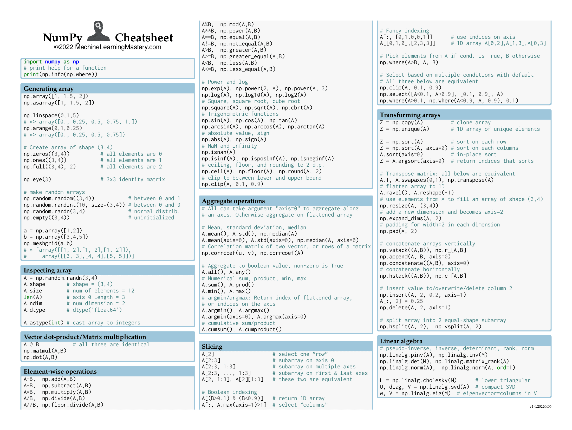
There are some cool features from NumPy that are worth mentioning as they are helpful for machine learning projects.

For instance, if we want to plot a 3D curve, we would compute $z=f(x,y)$ for a range of $x$ and $y$ and then plot the result in the $xyz$-space. We can generate the range with:

import numpy as np
x = np.linspace(-1, 1, 100)
y = np.linspace(-2, 2, 100)

For $z=f(x,y)=sqrt{1-x^2-(y/2)^2}$, we may need a nested for-loop to scan each value on arrays x and y and do the computation. But in NumPy, we can use meshgrid to expand two 1D arrays into two 2D arrays in the sense that by matching the indices, we get all the combinations as follows:

import matplotlib.pyplot as plt
import numpy as np

x = np.linspace(-1, 1, 100)
y = np.linspace(-2, 2, 100)

# convert vector into 2D arrays
xx, yy = np.meshgrid(x,y)
# computation on matching
z = np.sqrt(1 – xx**2 – (yy/2)**2)

fig = plt.figure(figsize=(8,8))
ax = plt.axes(projection=’3d’)
ax.set_xlim([-2,2])
ax.set_ylim([-2,2])
ax.set_zlim([0,2])
ax.plot_surface(xx, yy, z, cmap=”cividis”)
ax.view_init(45, 35)
plt.show()

In the above, the 2D array xx produced by meshgrid() has identical values on the same column, and yy has identical values on the same row. Hence element-wise operations on xx and yy are essentially operations on the $xy$-plane. This is why it works and why we can plot the ellipsoid above.

Another nice feature in NumPy is a function to expand the dimension. Convolutional layers in the neural network usually expect 3D images, namely, pixels in 2D, and the different color channels as the third dimension. It works for color images using RGB channels, but we have only one channel in grayscale images. For example, the digits dataset in scikit-learn:

from sklearn.datasets import load_digits
images = load_digits()[“images”]
print(images.shape)

(1797, 8, 8)

This shows that there are 1797 images from this dataset, and each is in 8×8 pixels. This is a grayscale dataset that shows each pixel is a value of darkness. We add the 4th axis to this array (i.e., convert a 3D array into a 4D array) so each image is in 8x8x1 pixels:

…

# image has axes 0, 1, and 2, adding axis 3
images = np.expand_dims(images, 3)
print(images.shape)

(1797, 8, 8, 1)

A handy feature in working with the NumPy array is Boolean indexing and fancy indexing. For example, if we have a 2D array:

import numpy as np

X = np.array([
[ 1.299, 0.332, 0.594, -0.047, 0.834],
[ 0.842, 0.441, -0.705, -1.086, -0.252],
[ 0.785, 0.478, -0.665, -0.532, -0.673],
[ 0.062, 1.228, -0.333, 0.867, 0.371]
])

we can check if all values in a column are positive:

…
y = (X > 0).all(axis=0)
print(y)

array([ True, True, False, False, False])

This shows only the first two columns are all positive. Note that it is a length-5 one-dimensional array, which is the same size as axis 1 of array X. If we use this Boolean array as an index on axis 1, we select the subarray for only where the index is positive:

…
y = X[:, (X > 0).all(axis=0)
print(y)

array([[1.299, 0.332],
[0.842, 0.441],
[0.785, 0.478],
[0.062, 1.228]])

If a list of integers is used in lieu of the Boolean array above, we select from X according to the index matching the list. NumPy calls this fancy indexing. So below, we can select the first two columns twice and form a new array:

…
y = X[:, [0,1,1,0]]
print(y)

array([[1.299, 0.332, 0.332, 1.299],
[0.842, 0.441, 0.441, 0.842],
[0.785, 0.478, 0.478, 0.785],
[0.062, 1.228, 1.228, 0.062]])

Functions from SciPy

SciPy is a sister project of NumPy. Hence, you will mostly see SciPy functions expecting NumPy arrays as arguments or returning one. SciPy provides a lot more functions that are less commonly used or more advanced.

SciPy functions are organized under submodules. Some common submodules are:

scipy.cluster.hierarchy: Hierarchical clustering
scipy.fft: Fast Fourier transform
scipy.integrate: Numerical integration
scipy.interpolate: Interpolation and spline functions
scipy.linalg: Linear algebra
scipy.optimize: Numerical optimization
scipy.signal: Signal processing
scipy.sparse: Sparse matrix representation
scipy.special: Some exotic mathematical functions
scipy.stats: Statistics, including probability distributions

But never assume SciPy can cover everything. For time series analysis, for example, it is better to depend on the statsmodels module instead.

We have covered a lot of examples using scipy.optimize in other posts. It is a great tool to find the minimum of a function using, for example, Newton’s method. Both NumPy and SciPy have the linalg submodule for linear algebra, but those in SciPy are more advanced, such as the function to do QR decomposition or matrix exponentials.

Maybe the most used feature of SciPy is the stats module. In both NumPy and SciPy, we can generate multivariate Gaussian random numbers with non-zero correlation.

import numpy as np
from scipy.stats import multivariate_normal
import matplotlib.pyplot as plt

mean = [0, 0] # zero mean
cov = [[1, 0.8],[0.8, 1]] # covariance matrix
X1 = np.random.default_rng().multivariate_normal(mean, cov, 5000)
X2 = multivariate_normal.rvs(mean, cov, 5000)

fig = plt.figure(figsize=(12,6))
ax = plt.subplot(121)
ax.scatter(X1[:,0], X1[:,1], s=1)
ax.set_xlim([-4,4])
ax.set_ylim([-4,4])
ax.set_title(“NumPy”)

ax = plt.subplot(122)
ax.scatter(X2[:,0], X2[:,1], s=1)
ax.set_xlim([-4,4])
ax.set_ylim([-4,4])
ax.set_title(“SciPy”)

plt.show()

But if we want to reference the distribution function itself, it is best to depend on SciPy. For example, the famous 68-95-99.7 rule is referring to the standard normal distribution, and we can get the exact percentage from SciPy’s cumulative distribution functions:

from scipy.stats import norm
n = norm.cdf([1,2,3,-1,-2,-3])
print(n)
print(n[:3] – n[-3:])

[0.84134475 0.97724987 0.9986501 0.15865525 0.02275013 0.0013499 ]
[0.68268949 0.95449974 0.9973002 ]

So we see that we expect a 68.269% probability that values fall within one standard deviation from the mean in a normal distribution. Conversely, we have the percentage point function as the inverse function of the cumulative distribution function:

…
print(norm.ppf(0.99))

2.3263478740408408

So this means if the values are in a normal distribution, we expect a 99% probability (one-tailed probability) that the value will not be more than 2.32 standard deviations beyond the mean.

These are examples of how SciPy can give you an extra mile over what NumPy gives you.

Speeding Up with numba

NumPy is faster than native Python because many of the operations are implemented in C and use optimized algorithms. But there are times when we want to do something, but NumPy is still too slow.

It may help if you ask numba to further optimize it by parallelizing or moving the operation to GPU if you have one. You need to install the numba module first:

pip install numba

And it may take a while if you need to compile numba into a Python module. Afterward, if you have a function that is purely NumPy operations, you can add the numba decorator to speed it up:

import numba

@numba.jit(nopython=True)
def numpy_only_function(…)
…

What it does is use a just-in-time compiler to vectorize the operation so it can run faster. You can see the best performance improvement if your function is running many times in your program (e.g., the update function in gradient descent) because the overhead of running the compiler can be amortized.

For example, below is an implementation of the t-SNE algorithm to transform 784-dimensional data into 2-dimensional. We are not going to explain the t-SNE algorithm in detail, but it needs many iterations to converge. The following code shows how we can use numba to optimize the inner loop functions (and it demonstrates some NumPy usage as well). It takes a few minutes to finish. You may try to remove the @numba.jit decorators afterward. It will take a considerably longer time.

import datetime

import tensorflow as tf
import matplotlib.pyplot as plt
import numpy as np
import numba

def tSNE(X, ndims=2, perplexity=30, seed=0, max_iter=500, stop_lying_iter=100, mom_switch_iter=400):
“””The t-SNE algorithm

Args:
X: the high-dimensional coordinates
ndims: number of dimensions in output domain
Returns:
Points of X in low dimension
“””
momentum = 0.5
final_momentum = 0.8
eta = 200.0
N, _D = X.shape
np.random.seed(seed)

# normalize input
X -= X.mean(axis=0) # zero mean
X /= np.abs(X).max() # min-max scaled

# compute input similarity for exact t-SNE
P = computeGaussianPerplexity(X, perplexity)
# symmetrize and normalize input similarities
P = P + P.T
P /= P.sum()
# lie about the P-values
P *= 12.0
# initialize solution
Y = np.random.randn(N, ndims) * 0.0001
# perform main training loop
gains = np.ones_like(Y)
uY = np.zeros_like(Y)
for i in range(max_iter):
# compute gradient, update gains
dY = computeExactGradient(P, Y)
gains = np.where(np.sign(dY) != np.sign(uY), gains+0.2, gains*0.8).clip(0.1)
# gradient update with momentum and gains
uY = momentum * uY – eta * gains * dY
Y = Y + uY
# make the solution zero-mean
Y -= Y.mean(axis=0)
# Stop lying about the P-values after a while, and switch momentum
if i == stop_lying_iter:
P /= 12.0
if i == mom_switch_iter:
momentum = final_momentum
# print progress
if (i % 50) == 0:
C = evaluateError(P, Y)
now = datetime.datetime.now()
print(f”{now} – Iteration {i}: Error = {C}”)
return Y

@numba.jit(nopython=True)
def computeExactGradient(P, Y):
“””Gradient of t-SNE cost function

Args:
P: similarity matrix
Y: low-dimensional coordinates
Returns:
dY, a numpy array of shape (N,D)
“””
N, _D = Y.shape
# compute squared Euclidean distance matrix of Y, the Q matrix, and the normalization sum
DD = computeSquaredEuclideanDistance(Y)
Q = 1/(1+DD)
sum_Q = Q.sum()
# compute gradient
mult = (P – (Q/sum_Q)) * Q
dY = np.zeros_like(Y)
for n in range(N):
for m in range(N):
if n==m: continue
dY[n] += (Y[n] – Y[m]) * mult[n,m]
return dY

@numba.jit(nopython=True)
def evaluateError(P, Y):
“””Evaluate t-SNE cost function

Args:
P: similarity matrix
Y: low-dimensional coordinates
Returns:
Total t-SNE error C
“””
DD = computeSquaredEuclideanDistance(Y)
# Compute Q-matrix and normalization sum
Q = 1/(1+DD)
np.fill_diagonal(Q, np.finfo(np.float32).eps)
Q /= Q.sum()
# Sum t-SNE error: sum P log(P/Q)
error = P * np.log( (P + np.finfo(np.float32).eps) / (Q + np.finfo(np.float32).eps) )
return error.sum()

@numba.jit(nopython=True)
def computeGaussianPerplexity(X, perplexity):
“””Compute Gaussian Perplexity

Args:
X: numpy array of shape (N,D)
perplexity: double
Returns:
Similarity matrix P
“””
# Compute the squared Euclidean distance matrix
N, _D = X.shape
DD = computeSquaredEuclideanDistance(X)
# Compute the Gaussian kernel row by row
P = np.zeros_like(DD)
for n in range(N):
found = False
beta = 1.0
min_beta = -np.inf
max_beta = np.inf
tol = 1e-5

# iterate until we get a good perplexity
n_iter = 0
while not found and n_iter < 200:
# compute Gaussian kernel row
P[n] = np.exp(-beta * DD[n])
P[n,n] = np.finfo(np.float32).eps
# compute entropy of current row
# Gaussians to be row-normalized to make it a probability
# then H = sum_i -P[i] log(P[i])
# = sum_i -P[i] (-beta * DD[n] – log(sum_P))
# = sum_i P[i] * beta * DD[n] + log(sum_P)
sum_P = P[n].sum()
H = beta * (DD[n] @ P[n]) / sum_P + np.log(sum_P)
# Evaluate if entropy within tolerance level
Hdiff = H – np.log2(perplexity)
if -tol < Hdiff < tol:
found = True
break
if Hdiff > 0:
min_beta = beta
if max_beta in (np.inf, -np.inf):
beta *= 2
else:
beta = (beta + max_beta) / 2
else:
max_beta = beta
if min_beta in (np.inf, -np.inf):
beta /= 2
else:
beta = (beta + min_beta) / 2
n_iter += 1
# normalize this row
P[n] /= P[n].sum()
assert not np.isnan(P).any()
return P

@numba.jit(nopython=True)
def computeSquaredEuclideanDistance(X):
“””Compute squared distance
Args:
X: numpy array of shape (N,D)
Returns:
numpy array of shape (N,N) of squared distances
“””
N, _D = X.shape
DD = np.zeros((N,N))
for i in range(N-1):
for j in range(i+1, N):
diff = X[i] – X[j]
DD[j][i] = DD[i][j] = diff @ diff
return DD

(X_train, y_train), (X_test, y_test) = tf.keras.datasets.mnist.load_data()
# pick 1000 samples from the dataset
rows = np.random.choice(X_test.shape[0], 1000, replace=False)
X_data = X_train[rows].reshape(1000, -1).astype(“float”)
X_label = y_train[rows]
# run t-SNE to transform into 2D and visualize in scatter plot
Y = tSNE(X_data, 2, 30, 0, 500, 100, 400)
plt.figure(figsize=(8,8))
plt.scatter(Y[:,0], Y[:,1], c=X_label)
plt.show()

Further Reading

This section provides more resources on the topic if you are looking to go deeper.

API documentations

NumPy user guide
SciPy user guide
Numba documentation

Summary

In this tutorial, you saw a brief overview of the functions provided by NumPy and SciPy.

Specifically, you learned:

How to work with NumPy arrays
A few functions provided by SciPy to help
How to make NumPy code faster by using the JIT compiler from numba

The post Scientific Functions in NumPy and SciPy appeared first on Machine Learning Mastery.

Read MoreMachine Learning Mastery