

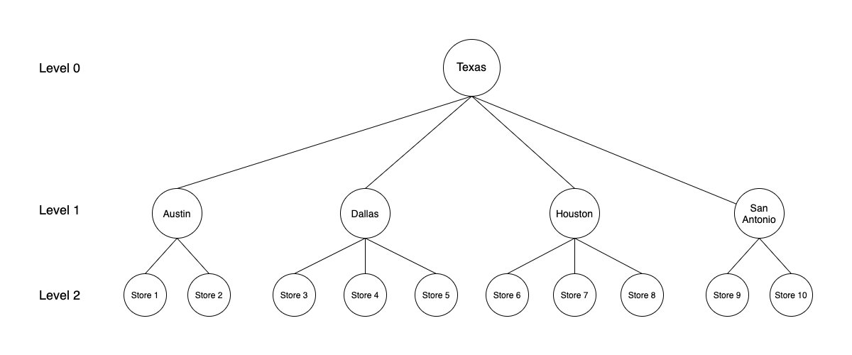
Time series forecasting is a common problem in machine learning (ML) and statistics. Some common day-to-day use cases of time series forecasting involve predicting product sales, item demand, component supply, service tickets, and all as a function of time. More often than not, time series data follows a hierarchical aggregation structure. For example, in retail, weekly sales for a Stock Keeping Unit (SKU) at a store can roll up to different geographical hierarchies at the city, state, or country level. In these cases, we must make sure that the sales estimates are in agreement when rolled up to a higher level. In these scenarios, Hierarchical Forecasting is used. It is the process of generating coherent forecasts (or reconciling incoherent forecasts) that allows individual time series to be forecasted individually while still preserving the relationships within the hierarchy. Hierarchical time series often arise due to various smaller geographies combining to form a larger one. For example, the following figure shows the case of a hierarchical structure in time series for store sales in the state of Texas. Individual store sales are depicted in the lowest level (level 2) of the tree, followed by sales aggregated on the city level (level 1), and finally all of the city sales aggregated on the state level (level 0).
In this post, we will first review the concept of hierarchical forecasting, including different reconciliation approaches. Then, we will take an example of demand forecasting on synthetic retail data to show you how to train and tune multiple hierarchical time series models. We will also perform hyper-parameter combinations using the scikit-hts toolkit on Amazon SageMaker, which is the most comprehensive and fully managed ML service. Amazon SageMaker lets data scientists and developers quickly and easily build and train ML models, and then directly deploy them into a production-ready hosted environment.
The forecasts at all of the levels must be coherent. The forecast for Texas in the previous figure should break down accurately into forecasts for the cities, and the forecasts for cities should also break down accurately for forecasts on the individual store level. There are various approaches to combining and breaking forecasts at different levels. The most common of these methods, as discussed in detail in Hyndman and Athanasopoulos, are as follows:
Bottom-Up:
In this method, the forecasts are carried out at the bottom-most level of the hierarchy, and then summed going up. For example, in the preceding figure, by using the bottom-up method, the time series’ for the individual stores (level 2) are used to build forecasting models. The outputs of individual models are then summed to generate the forecast for the cities. For example, forecasts for Store 1 and Store 2 are summed to get the forecasts for Austin. Finally, forecasts for all of the cities are summed to generate the forecasts for Texas.
Top-down:
In top-down approaches, the forecast is first generated for the top level (Texas in the preceding figure) and then disaggregated down the hierarchy. Disaggregate proportions are used in conjunction with the top level forecast to generate forecasts at the bottom level of the hierarchy. There are multiple methods to generate these disaggregate proportions, such as average historical proportions, proportions of the historical averages, and forecast proportions. These methods are briefly described in the following section. For a detailed discussion, please see Hyndman and Athanasopoulos.
Average historical proportions:
In this method, the bottom level series is generated by using the average of the historical proportions of the series at the bottom level (stores in the figure preceding), relative to the series at the top level (Texas in the preceding figure).
Proportions of the historical averages:
The average historical value of the series at the bottom level (stores in the preceding figure) relative to the average historical value of the series at the top level (Texas in the preceding figure) is used as the disaggregation proportion.
While both of the preceding top-down approaches are simple to implement and use, they are generally very accurate for the top level and are less accurate for lower levels. This is due to the loss of information and the inability to take advantage of characteristics of individual time series at lower levels. Furthermore, these methods also fail to account for how the historical proportions may change over time.
Forecast proportions:
In this method, instead of historical data, proportions based on forecasts are used for disaggregation. Forecasts are first generated for each individual series. These forecasts are not used directly, since they are not coherent at different levels of hierarchy. At each level, the proportions of these initial forecasts to that of the aggregate of all initial forecasts at the level are calculated. Then, these forecast proportions are used to disaggregate the top level forecast into individual forecasts at various levels. This method does not rely on outdated historical proportions and uses the current data to calculate the appropriate proportions. Due to this reason, forecast proportions often result in much more accurate forecasts as compared to the average historical proportions and proportions of the historical averages top-down approaches.
Middle-out:
In this method, forecasts are first generated for all of the series at a “middle level” (for example, Austin, Dallas, Houston, and San Antonio in the preceding figure). From these forecasts, the bottom-up approach is used to generate the aggregated forecasts for the levels above this middle level. For the levels below the middle level, a top-down approach is used.
Ordinary least squares (OLS):
In OLS, a least squares estimator is used to compute the reconciliation weights needed for generating coherent forecasts.
Solution overview
In this post, we take the example of demand forecasting on synthetic retail data to fine tune multiple hierarchical time series models across algorithms and hyper-parameter combinations. We are using the scikit-hts toolkit on Amazon SageMaker, which is the most comprehensive and fully managed ML service. SageMaker lets data scientists and developers quickly and easily build and train ML models, and then directly deploy them into a production-ready hosted environment.
First, we will show you how to setup scikit-hts on SageMaker using the SKLearn estimator, train multiple models using the SKLearn estimator, and track and organize experiments using SageMaker Experiments. We will walk you through the following steps:
Prerequisites
Prepare Time Series Data
Setup the scikit-hts training script
Setup the SKLearn Estimator
Setup Amazon SageMaker Experiment and Trials
Evaluate metrics and select a winning candidate
Runtime series forecasts
Visualize the forecasts:
Visualization at Region Level
Visualization at State Level
Prerequisites
The following is needed to follow along with this post and run the associated code:
An AWS account for running the code
Amazon Simple Storage Service (S3)
Amazon SageMaker (Notebook Instance or SageMaker Studio)
Amazon CloudWatch
An AWS Identity and Access Management (IAM) role to access Amazon SageMaker, S3, and CloudWatch
The code and associated dataset
Compatible versions of Amazon SageMaker’s SKLearn container (0.23-1), scikit-learn (0.23-1), scikit-hts (0.5.11)
Prepare Time Series Data
For this post, we will use synthetic retail clothing data to perform feature engineering steps to clean data. Then, we will convert the data into hierarchical representations as required by the scikit-hts package.
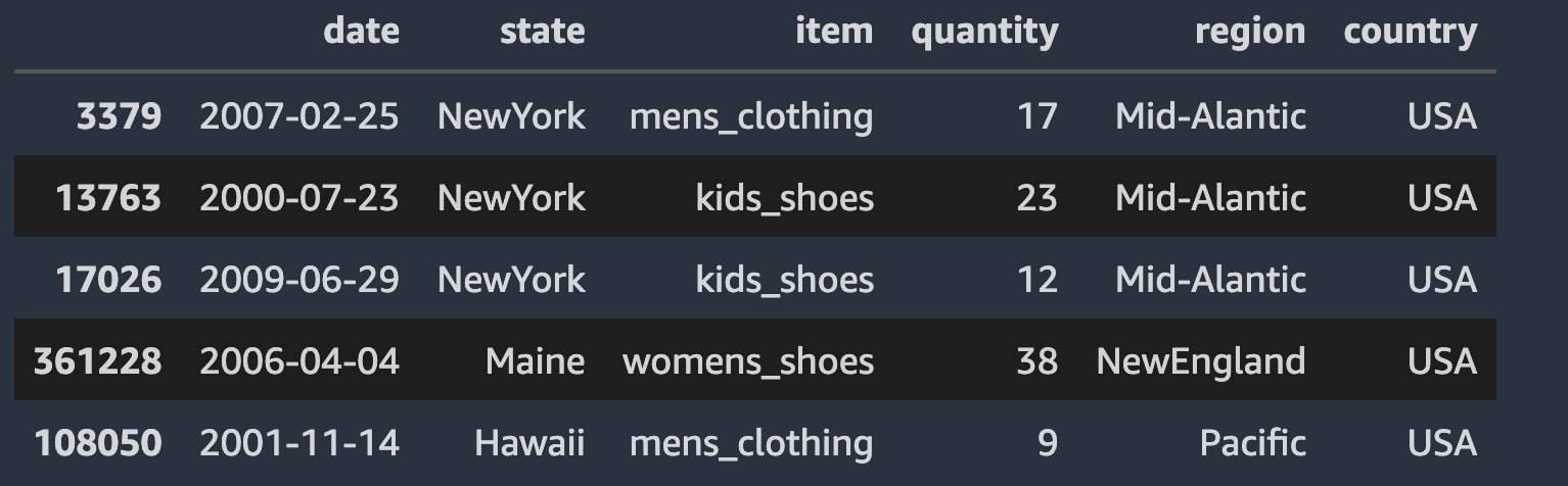
The retail clothing data is the time series daily quantity of sales data for six item categories: men’s clothing, men’s shoes, women’s clothing, women’s shoes, kids’ clothing, and kids’ shoes. The date range for the data is 11/25/1997 through 7/28/2009. Each row of the data corresponds to the quantity of sales for an item category in a state (total of 18 US states) for a specific date in the date range. Furthermore, the 18 states are also categorized into five US regions. The data is synthetically generated using repeatable patterns (for seasonality) with random noise added for each day.
First, let’s read the data into a Pandas DataFrame.
Define the S3 bucket and folder locations to store the test and training data. This should be within the same region as SageMaker Studio.
Now, let’s divide the raw data into train and test samples, and save them in their respective S3 folder locations using the Pandas DataFrame query function. We can check the first few entries of the train and test dataset. Both datasets should have the same fields, as in the following code:
Convert data into Hierarchical Representation
scikit-hts requires that each column in our DataFrame is a time series of its own, and for all hierarchy levels. To acheive this, we have created a dataset_prep.py script, which performs the following steps:
Transform the dataset into a column-oriented one.
Create the hierarchy representation as a dictionary.
For a complete description of how this is done under the hood, and for a sense of what the API accepts, see the scikit-hts’ docs.
Once we have created the hierarchy represenation as a dictionary, then we can visualize the data as a tree structure:
Setup the scikit-hts training script
We use a Python entry script to import the necessary SKLearn libraries, set up the scikit-hts estimators using the model packages for our algorithms of interest, and pass in our algorithm and hyper-parameter preferences from the SKLearn estimator that we set up in the notebook. In this post and associated code, we show the implementation and results for the bottom-up approach and the top-down approach with the average historical proportions division method. Note that the user can change these to select different hierarchical methods from the package. In addition, for the hyperparameters, we used additive and multiplicative seasonality with both the bottom-up and top-down approaches. The script uses the train and test data files that we uploaded to Amazon S3 to create the corresponding SKLearn datasets for training and evaluation. When training is complete, the script runs an evaluation to generate metrics, which we use to choose a winning model. For further analysis, the metrics are also available via the SageMaker trial component analytics (discussed later in this post). Then, the model is serialized for storage and future retrieval.
For more details, refer to the entry script “train.py” that is available in the GitHub repo. From the accompanying notebook, you can also run the cell in Step 3 to review the script. The following code shows the train function calling HTSRegressor with the Prophet algorithm along with the hierarchical method and seasonality mode:
Setup Amazon SageMaker Experiment and Trials
SageMaker Experiments automatically tracks the inputs, parameters, configurations, and results of your iterations as trials. You can assign, group, and organize these trials into experiments. SageMaker Experiments is integrated with SageMaker Studio. This provides a visual interface to browse your active and past experiments, compare trials on key performance metrics, and identify the best-performing models. SageMaker Experiments comes with its own Experiments SDK, which makes the analytics capabilities easily accessible in SageMaker notebooks. Because SageMaker Experiments enables tracking of all the steps and artifacts that go into creating a model, you can quickly revisit the origins of a model when you’re troubleshooting issues in production or auditing your models for compliance verifications. You can create your experiment with the following code:
For each job, we define a new Trial component within that experiment:
Next, we define an experiment config, which is a dictionary that we pass into the fit() method of SKLearn estimator later on. This makes sure that the training job is associated with that experiment and trial. For the full code block for this step, refer to the accompanying notebook. In the notebook, we use the bottom-up and top-down (with average historical proportions) approaches, along with additive and multiplicative seasonality as the seasonality hyperparameter values. This lets us train four different models. The code can be modified easily to use the rest of the hierarchical forecasting approaches discussed in the previous sections, since they are also implemented in scikit-hts package.
Creating the SKLearn estimator
You can run SKLearn training scripts on SageMaker’s fully managed training environment by creating an SKLearn estimator. Let’s set up the actual training runs with a combination of parameters and encapsulate the training jobs within SageMaker experiments.
We will use scikit-hts to fit the FBProphet model in our data and compare the results.
FBProphet
daily_seasonality: By default, daily seasonality is set to False, thereby explicitly changing it to True.
changepoint_prior_scale: If the trend changes are being overfit (too much flexibility) or underfit (not enough flexibility), you can adjust the strength of the sparse prior using the input argument changepoint_prior_scale. By default, this parameter is set to 0.05. Increasing it will make the trend more flexible.
See the following code:
After specifying our estimator with all of the necessary hyperparameters, we can train it using our training dataset. We train it by invoking the fit() method of the SKLearn estimator. We pass the location of the train and test data, as well as the experiment configuration. The training algorithm returns a fitted model that we can use to construct forecasts. See the following code:
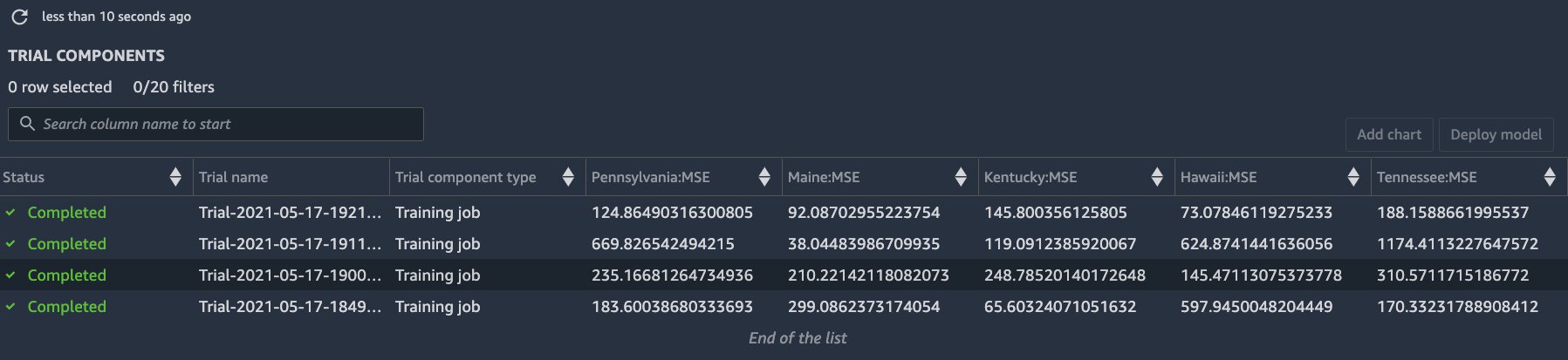
We start four training jobs in this case corresponding to the combinations of two hierarchical forecasting methods and two seasonality modes. These jobs are run in parallel using SageMaker training. The average runtime for these training jobs in this example was approximately 450 seconds on ml.m4.xlarge instances. You can review the job parameters and metrics from the trial component view in SageMaker Studio (see the following screenshot):
Evaluate metrics and select a winning candidate
Amazon SageMaker Studio provides an experiments browser that you can use to view the lists of experiments, trials, and trial components. You can choose one of these entities to view detailed information about the entity, or choose multiple entities for comparison. For more details, refer to the documentation. Once the training jobs are running, we can use the experiment view in Studio (see the following screenshot) or the ExperimentAnalytics module to track the status of our training jobs and their metrics.
In the training script, we used SKLearn Metrics to calculate the mean_squared_error (MSE) and stored it in the experiment. We can access the recorded metrics via the ExperimentAnalytics function and convert it to a Pandas DataFrame. The training job with the lowest Mean Squared Error (MSE) is the winner.
Let’s select the winner model and download it for running forecasts:
Runtime series forecasts
Now, we will load the model and make forecasts 90 days in future:
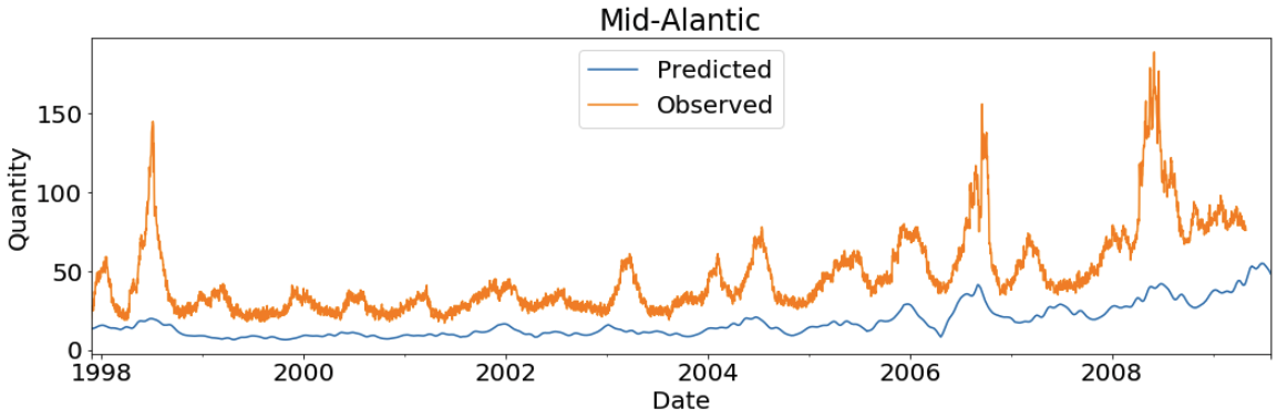
Visualize the forecasts
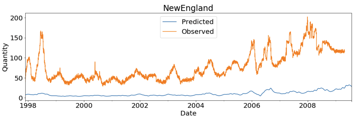
Let’s visualize the model results and fitted values for all of the states:
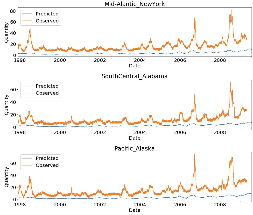
Visualization at Region Level
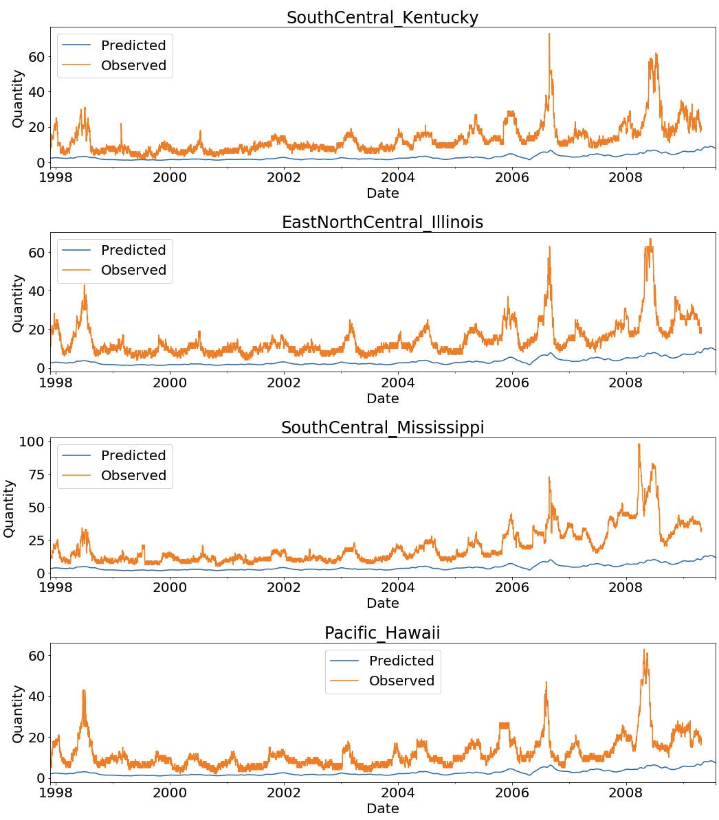
Visualization at State Level
The following screenshot is for some of the states. For a full list of state visualizations, execute the visualization section of the notebook.
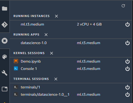
Clean up
Make sure to shut down the studio notebook. You can reach the Running Terminals and Kernels pane on the left side of Amazon SageMaker Studio with the icon. The Running Terminals and Kernels pane consists of four sections. Each section lists all of the resources of that type. You can shut down each resource individually or shut down all of the resources in a section at the same time.
Conclusion
Hierarchical forecasting is important where time series data can be grouped or aggregated at various levels in a hierarchical fashion. For accurate forecasting/prediction at various levels of hierarchy, methods that generate coherent forecasts at these different levels are needed. In this post, we demonstrated how we can leverage Amazon SageMaker’s training capabilities to carry out hierarchical forecasting. We used synthetic retail data and showed how to train hierarchical forecasting models using the scikit-hts package. We used the FBProphet model along with bottom-up and top-down (average historic proportions) hierarchical aggregation and disaggregation methods (see code). Furthermore, we used SageMaker Experiments to train multiple models and picked the best model out of the four trained models. While we only demonstrated this approach on a synthetic retail dataset, the code provided can easily be used with any time-series dataset that exhibits a similar hierarchical structure.
References
Training, debugging and running time series forecasting models with the GluonTS toolkit on Amazon SageMaker
Forecasting: Principles and Practice (2nd ed) by Rob J. Hyndman and George Athanasopoulos
Scikit-hts documentation
Scikit-hts examples
About the Authors
Mani Khanuja is an Artificial Intelligence and Machine Learning Specialist SA at Amazon Web Services (AWS). She helps customers use machine learning to solve their business challenges with AWS. She spends most of her time diving deep and teaching customers on AI/ML projects related to computer vision, natural language processing, forecasting, ML at the edge, and more. She is passionate about ML at the edge. She has created her own lab with a self-driving kit and prototype manufacturing production line, where she spends a lot of her free time.
Farooq Sabir is a Senior Artificial Intelligence and Machine Learning Specialist Solutions Architect at AWS. He holds PhD and MS degrees in Electrical Engineering from The University of Texas at Austin and a MS in Computer Science from Georgia Institute of Technology. He has over 15 years of work experience and also likes to teach and mentor college students. At AWS, he helps customers formulate and solve their business problems in data science, machine learning, computer vision, artificial intelligence, numerical optimization and related domains. Based in Dallas, Texas, he and his family love to travel and make long road trips.
Neha Gupta is a Solutions Architect at AWS and has 16 years of experience as a Database architect/ DBA. Apart from work, she’s outdoorsy and loves to dance.
Read MoreAWS Machine Learning Blog