Last Updated on February 26, 2022

Working on a machine learning project means we need to experiment. Having a way to configure your script easily will help you move faster. In Python, we have a way to adapt the code from command line. In this tutorial, we are going to see how we can leverage the command line arguments to a Python script to help you work better in your machine learning project.

After finishing this tutorial, you will learn

Why we would like to control a Python script in command line
How we can work in a command line efficiently

Let’s get started.

Overview

This tutorial is in three parts, they are

Running a Python script in command line
Working on the command line
Alternative to command line arguments

Running a Python script in command line

There are many ways to run a Python script. Someone may run it as part of a Jupyter notebook. Someone may run it in an IDE. But in all platforms, it is always possible to run a Python script in command line. In Windows, you have the command prompt or PowerShell (or even better, the Windows Terminal). In macOS or Linux, you have the Terminal or xterm. Running a Python script in command line is powerful because you can pass in additional parameter to the script.

The following script allows us to pass in values from the command line into Python:

import sys

n = int(sys.argv[1])
print(n+1)

When we save these few lines into a file, and run it in command line with an argument:

$ python commandline.py 15
16

you will see it takes our argument, convert it into integer, add one into it and print. The list sys.argv contains the name of our script and all the arguments (all strings), which in the above case, it is [“commandline.py”, “15”].

When you run a command line with more complicated set of arguments, it takes some effort to process the list sys.argv. Therefore Python provided the library argparse to help. This is to assume GNU-style, which can be explained using the following example:

rsync -a -v –exclude=”*.pyc” -B 1024 –ignore-existing 192.168.0.3:/tmp/ ./

The optional arguments are introduced by “-” or “–“, which a single hyphen is to carry a single character “short option” (such as -a, -B and -v above), and two hyphens are for multiple characters “long options” (such as –exclude and –ignore-existing above). The optional arguments may have additional parameters, such as in -B 1024 or –exclude=”*.pyc”, the 1024 and “*.pyc” are parameters to -B and –exclude respectively. Additionally, we may also have compulsory arguments, which we just put them into the command line. The part 192.168.0.3:/tmp/ and ./ above are examples. The order of compulsory arguments are important. For example, the rsync command above will copy files from 192.168.0.3:/tmp/ to ./ instead of the other way round.

The following is to replicate the above example in Python using argparse:

import argparse

parser = argparse.ArgumentParser(description=”Just an example”,
formatter_class=argparse.ArgumentDefaultsHelpFormatter)
parser.add_argument(“-a”, “–archive”, action=”store_true”, help=”archive mode”)
parser.add_argument(“-v”, “–verbose”, action=”store_true”, help=”increase verbosity”)
parser.add_argument(“-B”, “–block-size”, help=”checksum blocksize”)
parser.add_argument(“–ignore-existing”, action=”store_true”, help=”skip files that exist”)
parser.add_argument(“–exclude”, help=”files to exclude”)
parser.add_argument(“src”, help=”Source location”)
parser.add_argument(“dest”, help=”Destination location”)
args = parser.parse_args()
config = vars(args)
print(config)

If you run the above script, you will see:

$ python argparse_example.py
usage: argparse_example.py [-h] [-a] [-v] [-B BLOCK_SIZE] [–ignore-existing] [–exclude EXCLUDE] src dest
argparse_example.py: error: the following arguments are required: src, dest

This is to mean you didn’t provide the compulsory arguments for src and dest. Perhaps the best reason to use argparse is to get a help screen for free if you provded -h or –help as the argument, like the following:

$ python argparse_example.py –help
usage: argparse_example.py [-h] [-a] [-v] [-B BLOCK_SIZE] [–ignore-existing] [–exclude EXCLUDE] src dest

Just an example

positional arguments:
src Source location
dest Destination location

optional arguments:
-h, –help show this help message and exit
-a, –archive archive mode (default: False)
-v, –verbose increase verbosity (default: False)
-B BLOCK_SIZE, –block-size BLOCK_SIZE
checksum blocksize (default: None)
–ignore-existing skip files that exist (default: False)
–exclude EXCLUDE files to exclude (default: None)

While the script did nothing real, if you provided the arguments as required, you will see this:

$ python argparse_example.py -a –ignore-existing 192.168.0.1:/tmp/ /home
{‘archive’: True, ‘verbose’: False, ‘block_size’: None, ‘ignore_existing’: True, ‘exclude’: None, ‘src’: ‘192.168.0.1:/tmp/’, ‘dest’: ‘/home’}

The parser object created by ArgumentParser() has a parse_args() method that reads sys.argv and returns a namespace object. This is an object that carries attributes and we can read using args.ignore_existing for example. But usually it is easier to handle if it is a Python dictionary. Hence we can convert it into one using vars(args).

Usually for all optional arguments, we provide the long option and sometimes also the short option. Then we can access the value provided from the command line using the long option as the key (with hyphen replaced with underscore, or the single-character short option as the key if we don’t have a long version). The “positional arguments” are not optional and their names are provided in the add_argument() function.

There are multiple types of arguments. For the optional arguments, sometimes we use them as a boolean flags but sometimes we expect them to bring in some data. In the above, we use action=”store_true” to make that option set to False by default and toggle to True if it is specified. For the other option such as -B above, by default it expects additional data to go following it.

We can further require an argument to be a specific type. For example the -B option above, we can make it to expect integer data by adding type like the following

parser.add_argument(“-B”, “–block-size”, type=int, help=”checksum blocksize”)

and if we provided the wrong type, argparse will help terminate our program with an informative error message:

python argparse_example.py -a -B hello –ignore-existing 192.168.0.1:/tmp/ /home
usage: argparse_example.py [-h] [-a] [-v] [-B BLOCK_SIZE] [–ignore-existing] [–exclude EXCLUDE] src dest
argparse_example.py: error: argument -B/–block-size: invalid int value: ‘hello’

Working on the command line

Empowering your Python script with command line arguments can bring it to a new level of reusability. First, let’s look at a simple example on fitting an ARIMA model to GDP time series. World Bank collected historical GDP data of many countries. We can make use of the pandas_datareader package to read the data. If you haven’t installed it yet, you can use pip (or conda if you installed Anacronda) to install the package:

pip install pandas_datareader

The code for the GDP data that we use is NY.GDP.MKTP.CN, we can get the data of a country in the form of a pandas DataFrame by

from pandas_datareader.wb import WorldBankReader

gdp = WorldBankReader(“NY.GDP.MKTP.CN”, “SE”, start=1960, end=2020).read()

and then we can tidy up the DataFrame a bit using the tools provided by pandas:

import pandas as pd

# Drop country name from index
gdp = gdp.droplevel(level=0, axis=0)
# Sort data in choronological order and set data point at year-end
gdp.index = pd.to_datetime(gdp.index)
gdp = gdp.sort_index().resample(“y”).last()
# Convert pandas DataFrame into pandas Series
gdp = gdp[“NY.GDP.MKTP.CN”]

then fitting an ARIMA model and use the model for prediction is not difficult. In the following, we fit using the first 40 data points and forecast for next 3. Then compare the forecast with the actual in terms of relative error:

import statsmodels.api as sm

model = sm.tsa.ARIMA(endog=gdp[:40], order=(1,1,1)).fit()
forecast = model.forecast(steps=3)
compare = pd.DataFrame({“actual”:gdp, “forecast”:forecast}).dropna()
compare[“rel error”] = (compare[“forecast”] – compare[“actual”])/compare[“actual”]
print(compare)

Putting it all together, and a little polishing, the following is the complete code:

import warnings
warnings.simplefilter(“ignore”)

from pandas_datareader.wb import WorldBankReader
import statsmodels.api as sm
import pandas as pd

series = “NY.GDP.MKTP.CN”
country = “SE” # Sweden
length = 40
start = 0
steps = 3
order = (1,1,1)

# Read the GDP data from WorldBank database
gdp = WorldBankReader(series, country, start=1960, end=2020).read()
# Drop country name from index
gdp = gdp.droplevel(level=0, axis=0)
# Sort data in choronological order and set data point at year-end
gdp.index = pd.to_datetime(gdp.index)
gdp = gdp.sort_index().resample(“y”).last()
# Convert pandas dataframe into pandas series
gdp = gdp[series]
# Fit arima model
result = sm.tsa.ARIMA(endog=gdp[start:start+length], order=order).fit()
# Forecast, and calculate the relative error
forecast = result.forecast(steps=steps)
df = pd.DataFrame({“Actual”:gdp, “Forecast”:forecast}).dropna()
df[“Rel Error”] = (df[“Forecast”] – df[“Actual”]) / df[“Actual”]
# Print result
with pd.option_context(‘display.max_rows’, None, ‘display.max_columns’, 3):
print(df)

This script prints the following output

Actual Forecast Rel Error
2000-12-31 2408151000000 2.367152e+12 -0.017025
2001-12-31 2503731000000 2.449716e+12 -0.021574
2002-12-31 2598336000000 2.516118e+12 -0.031643

The above code is short but we made it flexible enough by holding some parameters in variables. We can change the above code to use argparse so we can change some parameters from the command line, as follows:

from argparse import ArgumentParser, ArgumentDefaultsHelpFormatter
import warnings
warnings.simplefilter(“ignore”)

from pandas_datareader.wb import WorldBankReader
import statsmodels.api as sm
import pandas as pd

# Parse command line arguments
parser = ArgumentParser(formatter_class=ArgumentDefaultsHelpFormatter)
parser.add_argument(“-c”, “–country”, default=”SE”, help=”Two-letter country code”)
parser.add_argument(“-l”, “–length”, default=40, type=int, help=”Length of time series to fit the ARIMA model”)
parser.add_argument(“-s”, “–start”, default=0, type=int, help=”Starting offset to fit the ARIMA model”)
args = vars(parser.parse_args())

# Set up parameters
series = “NY.GDP.MKTP.CN”
country = args[“country”]
length = args[“length”]
start = args[“start”]
steps = 3
order = (1,1,1)

# Read the GDP data from WorldBank database
gdp = WorldBankReader(series, country, start=1960, end=2020).read()
# Drop country name from index
gdp = gdp.droplevel(level=0, axis=0)
# Sort data in choronological order and set data point at year-end
gdp.index = pd.to_datetime(gdp.index)
gdp = gdp.sort_index().resample(“y”).last()
# Convert pandas dataframe into pandas series
gdp = gdp[series]
# Fit arima model
result = sm.tsa.ARIMA(endog=gdp[start:start+length], order=order).fit()
# Forecast, and calculate the relative error
forecast = result.forecast(steps=steps)
df = pd.DataFrame({“Actual”:gdp, “Forecast”:forecast}).dropna()
df[“Rel Error”] = (df[“Forecast”] – df[“Actual”]) / df[“Actual”]
# Print result
with pd.option_context(‘display.max_rows’, None, ‘display.max_columns’, 3):
print(df)

If we run the code above in a command line, we can see it can now accept arguments:

$ python gdp_arima.py –help
usage: gdp_arima.py [-h] [-c COUNTRY] [-l LENGTH] [-s START]

optional arguments:
-h, –help show this help message and exit
-c COUNTRY, –country COUNTRY
Two-letter country code (default: SE)
-l LENGTH, –length LENGTH
Length of time series to fit the ARIMA model (default: 40)
-s START, –start START
Starting offset to fit the ARIMA model (default: 0)
$ python gdp_arima.py
Actual Forecast Rel Error
2000-12-31 2408151000000 2.367152e+12 -0.017025
2001-12-31 2503731000000 2.449716e+12 -0.021574
2002-12-31 2598336000000 2.516118e+12 -0.031643
$ python gdp_arima.py -c NO
Actual Forecast Rel Error
2000-12-31 1507283000000 1.337229e+12 -0.112821
2001-12-31 1564306000000 1.408769e+12 -0.099429
2002-12-31 1561026000000 1.480307e+12 -0.051709

In the last command above, we pass in -c NO to apply the same model to the GDP data of Norway (NO) instead of Sweden (SE). Hence, without the risk of messing up the code, we reused our code to a different dataset.

The power of introducing command line argument is that we can test out our code with varying parameters easily. For example, we want to see if ARIMA(1,1,1) model is a good model for predicting GDP and we want to verify with different time window of the nordic countries:

Denmark (DK)
Finland (FI)
Iceland (IS)
Norway (NO)
Sweden (SE)

We want to check for the window of 40 years but with different starting points (since 1960, 1965, 1970, 1975). Depends on the OS, you can build a for loop in Linux and mac using the bash shell syntax:

for C in DK FI IS NO SE; do
for S in 0 5 10 15; do
python gdp_arima.py -c $C -s $S
done
done

or, as the shell syntax permits, we can put everything in one line:

for C in DK FI IS NO SE; do for S in 0 5 10 15; do python gdp_arima.py -c $C -s $S ; done ; done

or even better, give some information at each iteration of the loop, and we get our script run multiple times:

$ for C in DK FI IS NO SE; do for S in 0 5 10 15; do echo $C $S; python gdp_arima.py -c $C -s $S ; done; done
DK 0
Actual Forecast Rel Error
2000-12-31 1.326912e+12 1.290489e+12 -0.027449
2001-12-31 1.371526e+12 1.338878e+12 -0.023804
2002-12-31 1.410271e+12 1.386694e+12 -0.016718
DK 5
Actual Forecast Rel Error
2005-12-31 1.585984e+12 1.555961e+12 -0.018931
2006-12-31 1.682260e+12 1.605475e+12 -0.045644
2007-12-31 1.738845e+12 1.654548e+12 -0.048479
DK 10
Actual Forecast Rel Error
2010-12-31 1.810926e+12 1.762747e+12 -0.026605
2011-12-31 1.846854e+12 1.803335e+12 -0.023564
2012-12-31 1.895002e+12 1.843907e+12 -0.026963

…

SE 5
Actual Forecast Rel Error
2005-12-31 2931085000000 2.947563e+12 0.005622
2006-12-31 3121668000000 3.043831e+12 -0.024934
2007-12-31 3320278000000 3.122791e+12 -0.059479
SE 10
Actual Forecast Rel Error
2010-12-31 3573581000000 3.237310e+12 -0.094099
2011-12-31 3727905000000 3.163924e+12 -0.151286
2012-12-31 3743086000000 3.112069e+12 -0.168582
SE 15
Actual Forecast Rel Error
2015-12-31 4260470000000 4.086529e+12 -0.040827
2016-12-31 4415031000000 4.180213e+12 -0.053186
2017-12-31 4625094000000 4.273781e+12 -0.075958

If you’re using Windows, you can use the following syntax in command prompt:

for %C in (DK FI IS NO SE) do for %S in (0 5 10 15) do python gdp_arima.py -c $C -s $S

or the following in PowerShell:

foreach ($C in “DK”,”FI”,”IS”,”NO”,”SE”) { foreach ($S in 0,5,10,15) { python gdp_arima.py -c $C -s $S } }

both should produce the same result.

While we can put similar loop inside our Python script, sometimes it is easier if we can do it at the command line. It could be more convenient when we are exploring different options. Moreover, by taking the loop outside of the Python code, we can be assured that every time we run the script is independent because we will not share any variables between iterations.

Alternative to command line arguments

Using command line arguments is not the only way to pass in data to your Python script. At least, there are several other ways too:

using environment variables
using config files

Environment variables are features from your OS to keep small amount of data in memory. We can read environment variables in Python using the following syntax:

import os
print(os.environ[“MYVALUE”])

For example, in Linux, the above two-line script will work with the shell as follows

$ export MYVALUE=”hello”
$ python show_env.py
hello

and in Windows, the syntax inside command prompt is similar:

C:MLM> set MYVALUE=hello

C:MLM> python show_env.py
hello

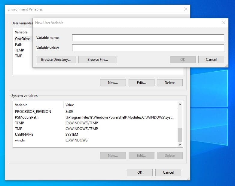
You may also add or edit environment variables in Windows using the dialog in Control Panel:

So we may keep the parameters to the script in some environment variables and let the script adapt its behavior like setting up command line arguments.

In case we have a lot of options to set, it is better to save the options to a file rather than overwhelming the command line. Depends on the format we chose, we can use the configparser or json module from Python for reading Windows INI format or JSON format respectively. We may also use the third party library PyYAML to read YAML format.

For the above example on running ARIMA model on GDP data, we can modify the code to use YAML config file:

import warnings
warnings.simplefilter(“ignore”)

from pandas_datareader.wb import WorldBankReader
import statsmodels.api as sm
import pandas as pd
import yaml

# Load config from YAML file
with open(“config.yaml”, “r”) as fp:
args = yaml.safe_load(fp)

# Set up parameters
series = “NY.GDP.MKTP.CN”
country = args[“country”]
length = args[“length”]
start = args[“start”]
steps = 3
order = (1,1,1)

# Read the GDP data from WorldBank database
gdp = WorldBankReader(series, country, start=1960, end=2020).read()
# Drop country name from index
gdp = gdp.droplevel(level=0, axis=0)
# Sort data in choronological order and set data point at year-end
gdp.index = pd.to_datetime(gdp.index)
gdp = gdp.sort_index().resample(“y”).last()
# Convert pandas dataframe into pandas series
gdp = gdp[series]
# Fit arima model
result = sm.tsa.ARIMA(endog=gdp[start:start+length], order=order).fit()
# Forecast, and calculate the relative error
forecast = result.forecast(steps=steps)
df = pd.DataFrame({“Actual”:gdp, “Forecast”:forecast}).dropna()
df[“Rel Error”] = (df[“Forecast”] – df[“Actual”]) / df[“Actual”]
# Print result
with pd.option_context(‘display.max_rows’, None, ‘display.max_columns’, 3):
print(df)

and the YAML config file is named as config.yaml, which its content is as follows:

country: SE
length: 40
start: 0

Then we can run the above code and obtaining the same result as before. The JSON counterpart is very similar, which we use the load() function from json module:

import json
import warnings
warnings.simplefilter(“ignore”)

from pandas_datareader.wb import WorldBankReader
import statsmodels.api as sm
import pandas as pd

# Load config from JSON file
with open(“config.json”, “r”) as fp:
args = json.load(fp)

# Set up parameters
series = “NY.GDP.MKTP.CN”
country = args[“country”]
length = args[“length”]
start = args[“start”]
steps = 3
order = (1,1,1)

# Read the GDP data from WorldBank database
gdp = WorldBankReader(series, country, start=1960, end=2020).read()
# Drop country name from index
gdp = gdp.droplevel(level=0, axis=0)
# Sort data in choronological order and set data point at year-end
gdp.index = pd.to_datetime(gdp.index)
gdp = gdp.sort_index().resample(“y”).last()
# Convert pandas dataframe into pandas series
gdp = gdp[series]
# Fit arima model
result = sm.tsa.ARIMA(endog=gdp[start:start+length], order=order).fit()
# Forecast, and calculate the relative error
forecast = result.forecast(steps=steps)
df = pd.DataFrame({“Actual”:gdp, “Forecast”:forecast}).dropna()
df[“Rel Error”] = (df[“Forecast”] – df[“Actual”]) / df[“Actual”]
# Print result
with pd.option_context(‘display.max_rows’, None, ‘display.max_columns’, 3):
print(df)

and the JSON config file, config.json would be

{
“country”: “SE”,
“length”: 40,
“start”: 0
}

You may learn more about the syntax of JSON and YAML for your project. But the idea here is that we can separate the data and algorithm for better reusability of our code.

Further reading

This section provides more resources on the topic if you are looking to go deeper.

Libraries

argparse module, https://docs.python.org/3/library/argparse.html
Pandas Data Reader, https://pandas-datareader.readthedocs.io/en/latest/
ARIMA in statsmodels, https://www.statsmodels.org/devel/generated/statsmodels.tsa.arima.model.ARIMA.html
configparser module, https://docs.python.org/3/library/configparser.html
json module, https://docs.python.org/3/library/json.html
PyYAML, https://pyyaml.org/wiki/PyYAMLDocumentation

Articles

Working with JSON, https://developer.mozilla.org/en-US/docs/Learn/JavaScript/Objects/JSON
YAML on Wikipedia, https://en.wikipedia.org/wiki/YAML

Books

Python Cookbook, third edition, by David Beazley and Brian K. Jones, https://www.amazon.com/dp/1449340377/

Summary

In this tutorial, you’ve see how we can make use of the command line for more efficient control of our Python script. Specifically, you learned

How we can pass in parameters to your Python script using the argparse module
How we can efficiently control the argparse-enabled Python script in a terminal under different OS
We can also use environment variables, or config files to pass in parameters to a Python script

The post Command line arguments for your Python script appeared first on Machine Learning Mastery.

Read MoreMachine Learning Mastery