Calculus in Action: Neural Networks

An artificial neural network is a computational model that approximates a mapping between inputs and outputs. 

It is inspired by the structure of the human brain, in that it is similarly composed of a network of interconnected neurons that propagate information upon receiving sets of stimuli from neighbouring neurons.

Training a neural network involves a process that employs the backpropagation and gradient descent algorithms in tandem. As we will be seeing, both of these algorithms make extensive use of calculus.

In this tutorial, you will discover how aspects of calculus are applied in neural networks. 

After completing this tutorial, you will know:

An artificial neural network is organized into layers of neurons and connections, where the latter are attributed a weight value each.
Each neuron implements a nonlinear function that maps a set of inputs to an output activation.
In training a neural network, calculus is used extensively by the backpropagation and gradient descent algorithms. 

Let’s get started. 

Tutorial Overview

This tutorial is divided into three parts; they are:

An Introduction to the Neural Network
The Mathematics of a Neuron
Training the Network

Prerequisites

For this tutorial, we assume that you already know what are:

Function approximation
Rate of change
Partial derivatives
The chain rule
The chain rule on more functions
Gradient descent

You can review these concepts by clicking on the links given above.

An Introduction to the Neural Network

Artificial neural networks can be considered as function approximation algorithms. 

In a supervised learning setting, when presented with many input observations representing the problem of interest, together with their corresponding target outputs, the artificial neural network will seek to approximate the mapping that exists between the two. 

A neural network is a computational model that is inspired by the structure of the human brain. 

– Page 65, Deep Learning, 2019. 

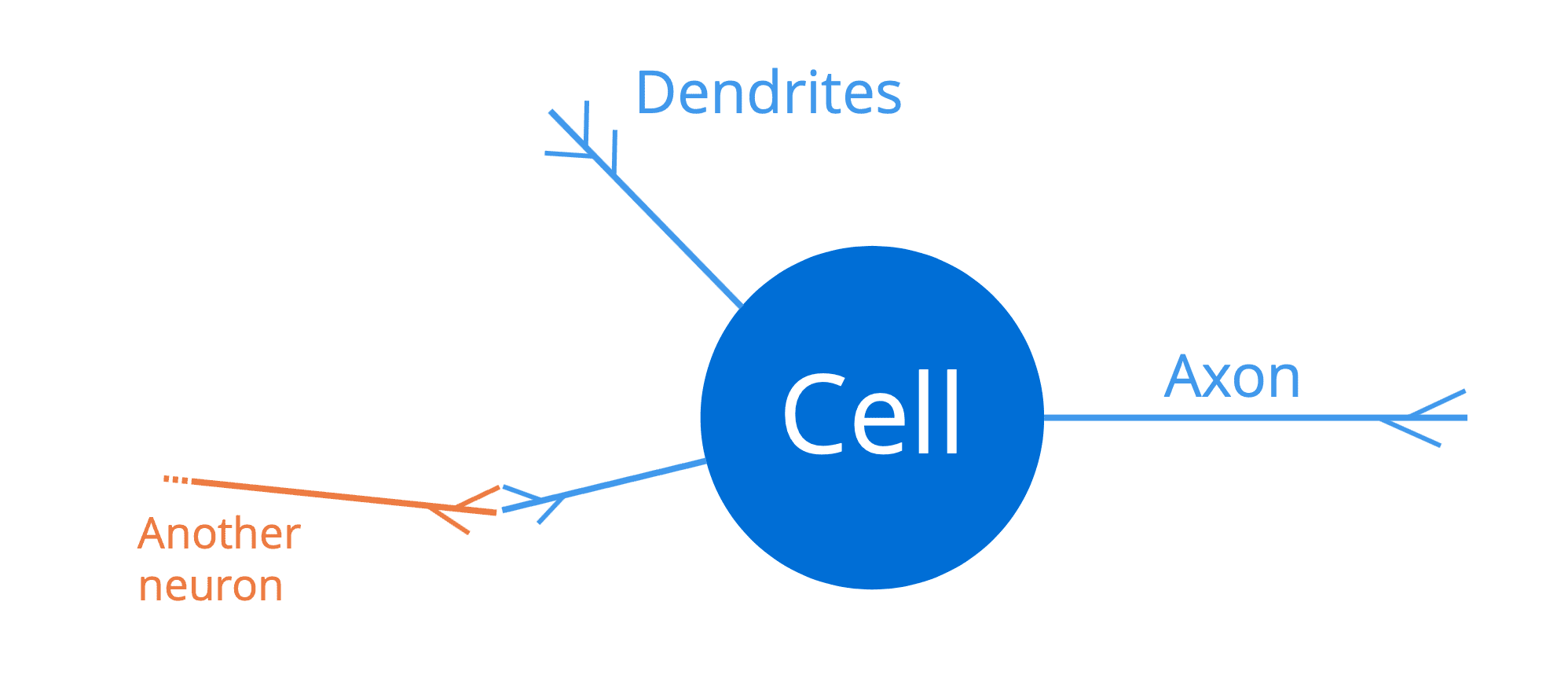
The human brain consists of a massive network of interconnected neurons (around one hundred billion of them), with each comprising a cell body, a set of fibres called dendrites, and an axon:

The dendrites act as the input channels to a neuron, whereas the axon acts as the output channel. Therefore, a neuron would receive input signals through its dendrites, which in turn would be connected to the (output) axons of other neighbouring neurons. In this manner, a sufficiently strong electrical pulse (also called an action potential) can be transmitted along the axon of one neuron, to all the other neurons that are connected to it. This permits signals to be propagated along the structure of the human brain. 

So, a neuron acts as an all-or-none switch, that takes in a set of inputs and either outputs an action potential or no output. 

– Page 66, Deep Learning, 2019.

An artificial neural network is analogous to the structure of the human brain, because (1) it is similarly composed of a large number of interconnected neurons that, (2) seek to propagate information across the network by, (3) receiving sets of stimuli from neighbouring neurons and mapping these to outputs, to be fed to the next layer of neurons. 

The structure of an artificial neural network is typically organised into layers of neurons (recall the depiction of a tree diagram). For example, the following diagram illustrates a fully-connected  neural network, where all the neurons in one layer are connected to all the neurons in the next layer:

The inputs are presented on the left hand side of the network, and the information propagates  (or flows) rightward towards the outputs at the opposite end. Since the information is, hereby, propagating in the forward direction through the network, then we would also refer to such a network as a feedforward neural network. 

The layers of neurons in between the input and output layers are called hidden layers, because they are not directly accessible. 

Each connection (represented by an arrow in the diagram) between two neurons is attributed a weight, which acts on the data flowing through the network, as we will see shortly. 

The Mathematics of a Neuron

More specifically, let’s say that a particular artificial neuron (or a perceptron, as Frank Rosenblatt had initially named it) receives n inputs, [x1, …, xn], where each connection is attributed a corresponding weight, [w1, …, wn]. 

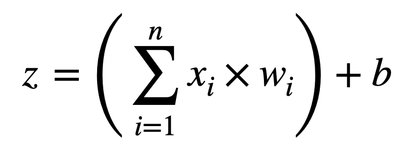
The first operation that is carried out multiplies the input values by their corresponding weight, and adds a bias term, b, to their sum, producing an output, z:

z = ((x1 × w1) + (x2 × w2) + … + (xn × wn)) + b

We can, alternatively, represent this operation in a more compact form as follows:

This weighted sum calculation that we have performed so far is a linear operation. If every neuron had to implement this particular calculation alone, then the neural network would be restricted to learning only linear input-output mappings. 

However, many of the relationships in the world that we might want to model are nonlinear, and if we attempt to model these relationships using a linear model, then the model will be very inaccurate. 

– Page 77, Deep Learning, 2019.

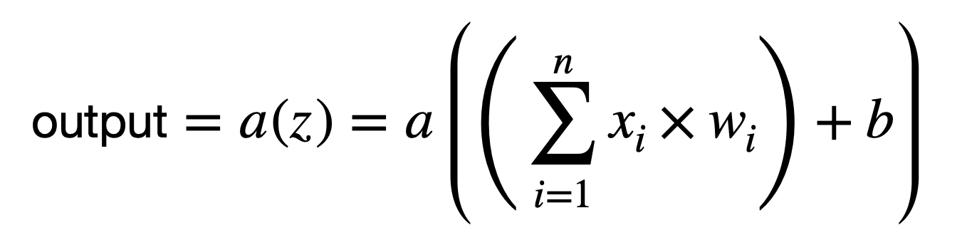
Hence, a second operation is performed by each neuron that transforms the weighted sum by the application of a nonlinear activation function, a(.): 

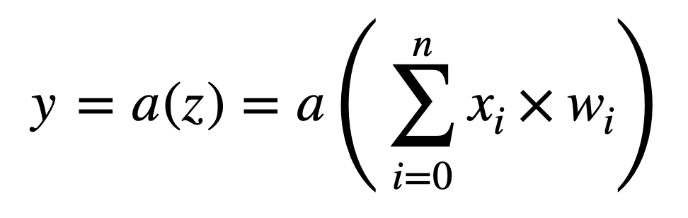
We can represent the operations performed by each neuron even more compactly, if we had to integrate the bias term into the sum as another weight, w0 (notice that the sum now starts from 0):

The operations performed by each neuron can be illustrated as follows:

Therefore, each neuron can be considered to implement a nonlinear function that maps a set of inputs to an output activation. 

Training the Network

Training an artificial neural network involves the process of searching for the set of weights that model best the patterns in the data. It is a process that employs the backpropagation and gradient descent algorithms in tandem. Both of these algorithms make extensive use of calculus. 

Each time that the network is traversed in the forward (or rightward) direction, the error of the network can be calculated as the difference between the output produced by the network and the expected ground truth, by means of a loss function (such as the sum of squared errors (SSE)). The backpropagation algorithm, then, calculates the gradient (or the rate of change) of this error to changes in the weights. In order to do so, it requires the use of the chain rule and partial derivatives. 

For simplicity, consider a network made up of two neurons connected by a single path of activation. If we had to break them open, we would find that the neurons perform the following operations in cascade:

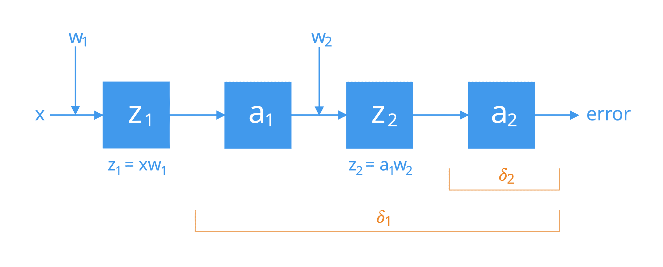
The first application of the chain rule connects the overall error of the network to the input, z2, of the activation function a2 of the second neuron, and subsequently to the weight, w2, as follows:

You may notice that the application of the chain rule involves, among other terms, a multiplication by the partial derivative of the neuron’s activation function with respect to its input, z2. There are different activation functions to choose from, such as the sigmoid or the logistic functions. If we had to take the logistic function as an example, then its partial derivative would be computed as follows:

Hence, we can compute 𝛿2 as follows:

Here, t2 is the expected activation, and in finding the difference between t2 and a2 we are, therefore, computing the error between the activation generated by the network and the expected ground truth. 

Since we are computing the derivative of the activation function, it should, therefore, be continuous and differentiable over the entire space of real numbers. In the case of deep neural networks, the error gradient is propagated backwards over a large number of hidden layers. This can cause the error signal to rapidly diminish to zero, especially if the maximum value of the derivative function is already small to begin with (for instance, the inverse of the logistic function has a maximum value of 0.25). This is known as the vanishing gradient problem. The ReLU function has been so popularly used in deep learning to alleviate this problem, because its derivative in the positive portion of its domain is equal to 1. 

The next weight backwards is deeper into the network and, hence, the application of the chain rule can similarly be extended to connect the overall error to the weight, w1, as follows:

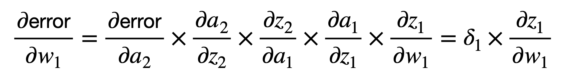
If we take the logistic function again as the activation function of choice, then we would compute 𝛿1 as follows:

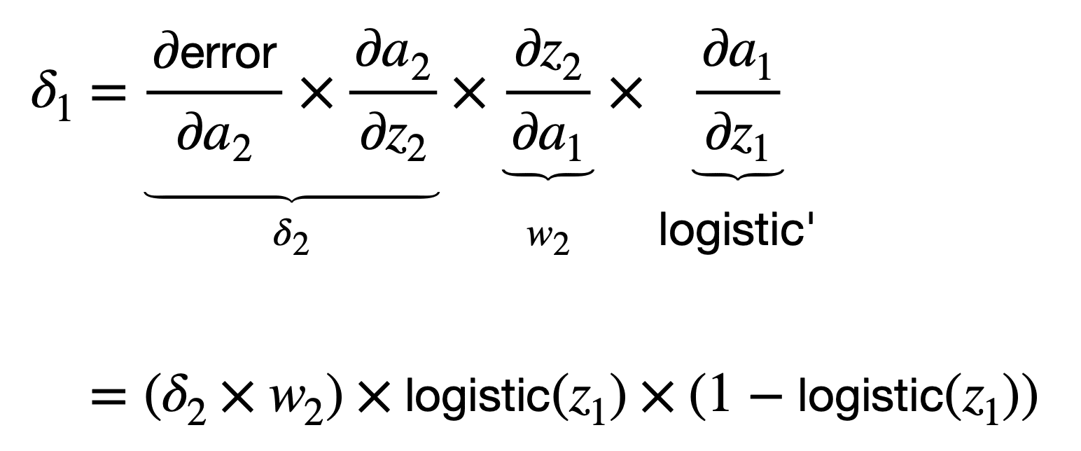
Once we have computed the gradient of the network error with respect to each weight, then the gradient descent algorithm can be applied to update each weight for the next forward propagation at time, t+1. For the weight, w1, the weight update rule using gradient descent would be specified as follows:

Even though we have hereby considered a simple network, the process that we have gone through can be extended to evaluate more complex and deeper ones, such convolutional neural networks (CNNs). 

If the network under consideration is characterised by multiple branches coming from multiple inputs (and possibly flowing towards multiple outputs), then its evaluation would involve the summation of different derivative chains for each path, similarly to how we have previously derived the generalized chain rule. 

Further Reading

This section provides more resources on the topic if you are looking to go deeper.

Books

Deep Learning, 2019.
Pattern Recognition and Machine Learning, 2016.

Summary

In this tutorial, you discovered how aspects of calculus are applied in neural networks. 

Specifically, you learned:

An artificial neural network is organized into layers of neurons and connections, where the latter are each attributed a weight value.
Each neuron implements a nonlinear function that maps a set of inputs to an output activation.
In training a neural network, calculus is used extensively by the backpropagation and gradient descent algorithms.

Do you have any questions?
Ask your questions in the comments below and I will do my best to answer.

The post Calculus in Action: Neural Networks appeared first on Machine Learning Mastery.

Read MoreMachine Learning Mastery