

This is a guest post by Russell Waterson, Knowledge Graph Engineer at Data Lens Ltd.
Customers use knowledge graphs to consolidate and integrate information assets and make them more readily available.
Building knowledge graphs by getting data from disparate existing data sources can be expensive, time-consuming, and complex. Project planning, project management, engineering, maintenance and release cycles all contribute to the complexity and time to build a platform to populate your knowledge graph database.
The Data Lens Ltd. team have been implementing Knowledge Graph solutions as a consultancy for 10 years, and have now released tooling to greatly reduce the time and effort required to build a Knowledge Graph.
Use Data Lens to make building a knowledge graph in Amazon Neptune faster and simpler. With no engineering, just configuration.
Solution overview
Here we use Data Lens on AWS Marketplace to export JSON content from an Amazon Simple Storage Service (Amazon S3) bucket, transform the JSON into RDF, and load the RDF data into Amazon Neptune.
To configure the transformation between JSON and RDF, Data Lens uses RML.
The Data Lens Structured File Lens uses an RML mapping configuration to transform the JSON data into RDF, and then the Data Lens Writer loads the RDF data into Amazon Neptune.
RML (RDF Mapping Language) is a language for expressing customized mappings from heterogeneous data structures and serializations to the RDF data model.
RDF (Resource Description Framework) is part of a family of World Wide Web Consortium (W3C) specifications for knowledge graph compatible data. The RDF 1.1 specification is supported by Amazon Neptune.
The following diagram illustrates our architecture.
To see this technology stack in action, we work through an example ingestion using a snippet of JSON source data. We cover the following topics:
An overview of the sample JSON input file
An overview of the mapping file used to define the transformation map from the source data to RDF
Calling the Structured File Lens to start the ingestion and transformation of the data
An overview of the transformed output RDF NQuads data
Calling the Lens Writer to start the ingestion and loading of the RDF data
An overview of the newly loaded RDF in Neptune using a simple SPARQL query within a Neptune Workbench using a Jupyter notebook
Reviewing additional features supported by Data Lens, including provenance and time series data, automation using Apache Kafka and AWS Lambda, custom functions, and more
Solution configuration and setup in AWS
To see how to setup all the services required to run this solution in AWS, see this related post:
Configure AWS services to build a knowledge graph in Amazon Neptune using Data Lens
Transform JSON data and upload to Neptune
To demonstrate an end-to-end solution of data transformation to Neptune ingestion, we consider a use case using JSON source data as the input. We use the Structured File Lens to process JSON files. In this post, we walk through the JSON input file, the RML mapping file used for the transformation, and the resulting RDF output file produced by the Lens. We then load this file into Neptune using the Lens Writer, and verify our results by using a simple SPARQL query within a Neptune Workbench using a Jupyter notebook.
JSON input source file
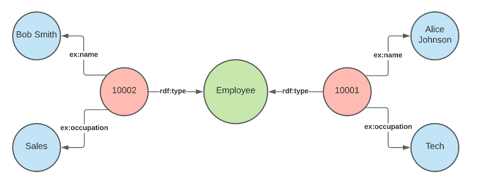
In the following JSON input file, we have two employees, each with data regarding their name and role in addition to an ID, which acts as a unique identifier for each record:
The aim is to transform this JSON into RDF data so that it can be easily identified, disambiguated, and interconnected. With the two employees, both with their unique identifier as the ID value, along with their name and occupation data, our resulting RDF looks like the following diagram.
RML mapping file
The mapping files, which we use to map data from the source to RDF, are written using RDF Mapping Language (RML). RML is defined as a superset of the W3C-recommended mapping language, R2RML. RML is a generic, scalable mapping language defined to express rules that map data in heterogeneous structures and serializations to the RDF data model. RML mappings are themselves RDF graphs and written down in Turtle syntax, therefore all mapping files created for use in the Lenses should be saved with the .ttl file extension.
The following mapping file example correlates to the previously explored JSON input file. In it, we create a single triples map that defines rules to generate zero or more RDF triples sharing the same subject:
In this section, we briefly explain the contents of the mapping file. For a more in-depth look at creating your own RML mapping file from scratch, as well as how to map other file types, see Manually Create a Mapping File in the Data Lens documentation.
A triples map consists of a logical source, a subject map, and zero or more predicate-object maps.
The logical source is made up of a reference to the input source, a reference formulation, and an iterator, with the following details:
The rml:source should always be inputSourceFile, and the suffix must match the file type you’re processing. For example:
JSON – inputSourceFile.json
XML – inputSourceFile.xml
CSV – inputSourceFile.csv
The reference formulation must also match the type of data you’re processing. For example:
JSON – rml:referenceFormulation ql:JSONPath;
XML – rml:referenceFormulation ql:SaXPath;
CSV – rml:referenceFormulation ql:CSV;
The iterator is a JSONPath identifying where to iterate over JSON objects in a file. For this post, we iterate over every element in the employees array: rml:iterator “$.[*].employees.[*]”.
RDF data is composed of triples. Triples are made up of three elements: subject, predicate, and object. For example, we can break down <http://example.com/10001> <rdfs:type> <http://example.com/Employee> as follows:
Subject – <http://example.com/10001>
Predicate – <rdfs:type>
Object – <http://example.com/Employee>
To create this triple from within our mapping file, we first need to define the subject of the triple in the mapping file by specifying the subjectMap:
Now that we have our subject and its class defined, we can create the rest of the predicates and objects related to the same subject. For example, to create the triple <http://example.com/10001> <ex:name> “Alice Johnson”, we need a predicateObjectMap to go with our subjectMap, which looks like the following code:
We can also define the object’s term type and data type. Furthermore, we can specify an object’s language, as demonstrated in the mapping of the triple <http://example.com/10001> <http://example.com/occupation> “Tech”@en-gb.
We now need a second predicateObjectMap, but this time we need to use simple JSONPath to access the occupation value due to the structure of the JSON source data. This results in a mapping that looks like the following:
Transform JSON into RDF using the Structured File Lens
Data Lens has designed several products tailored for specific use cases depending on how your source data is currently stored as well as its type. These individual products are called Lenses. Lenses are lightweight and highly scalable containers accessible from AWS Marketplace, ready to be integrated into your existing AWS Cloud architecture stack.
Now we have our input and mapping files ready, we can process our first transformation using the Structured File Lens. You can trigger the Lens several different ways, including using Apache Kafka as a message queue, or by having it be triggered by a Lambda function. For this post, we use the built-in REST API endpoint.
To trigger a file’s processing via the endpoint, we must call the process GET endpoint and specify the URL of a file to ingest. In response, we receive the URL of the newly generated RDF data file. This is explained more later in this post, however the structure and parameters for the GET request are simply as follows: http://<lens-address>/process?inputFileURL=<input-file-url>.
After a successful call to the RESTful endpoint, we receive a JSON response containing the processing report. One of the values in this report is the location of the successfully transformed RDF file. For following code is the resulting RDF file:
By default, the Lenses transform your data into NQuads using your mapping file, but they also support the ability to generate JSON-LD output files. For this post, we use the default NQuads transformation because we intend to upload the output data to Neptune.
In the resulting NQuads snippet, the Lens successfully transformed the input data using the mapping file. Looking closer, both records from the JSON were converted into three quads each, with the name, occupation, and type correlating exactly to what was previously defined in our mapping file. Each quad also has a named graph attached. These named graphs, which are unique for each file that is processed, are used for provenance.
Provenance
In addition to the output RDF files, the Lenses generate provenance files. These files are also NQuads RDF files that can subsequently be uploaded to Neptune. This is done using the Lens Writer, in exactly the same way as the output files are loaded, which we explore in the next section.
Within each Lens, time series data is supported as standard and every time a Lens ingests some data provenance, information is added. This means that you have a full record of data over time, allowing you to see what the state of the data was at any moment. The Data Lens Provenance Ontology expresses details about a Lens’s process. The model used to record provenance information extends the w3c standard PROV Ontology, PROV-O, and the RDF graph literals and named graphs (RDFG) using the OWL2 Web Ontology Language.
Load RDF into Neptune using the Lens Writer
Neptune is a fast, reliable, fully managed graph database service that makes it easy to build and run applications that work with highly connected datasets. The Lens Writer allows for fully automated ingestion of RDF data into a multitude of triplestores. This tool supports all the common knowledge graphs, including Neptune, and generic SPARQL support for less common knowledge graphs.
Now that our data has successfully been transformed into RDF in the form of an NQuads RDF file (with the .nq extension), we can start loading it into Neptune using the Lens Writer. Similarly to the Lenses, you can trigger the writer several ways. For this post, we use the same method as before, using the built-in REST API endpoint. We use a very similar structure as with the Lens, specifying the URL of the NQuads RDF file to ingest as http://<writer-address>/process?inputRdfURL=<input-rdf-file-url>.
After the RDF data is loaded into the Neptune instance, we can verify this by using the Neptune Workbench with Jupyter Notebooks. Jupyter Notebooks allows you to quickly and easily query your Neptune databases with a fully managed, interactive development environment with live code and narrative text. See the appendix at the end of this post for further instructions on setting up your notebook.
After we create the Jupyter notebook, we can run SPARQL queries against the knowledge graph. We use a simple select all query to see all the previously inserted RDF data in the graph. The query SELECT * WHERE { ?s ?p ?o } returns all the triples (subject-predicate-object) in the graph, which in our case is the six triples from our newly generated NQuads file.
The following screenshot shows the results of the SPARQL query; the RDF data has successfully been loaded into our Neptune knowledge graph.
This example covered a single small sample RDF file. If you have multiple large files, you can scale the Lens Writer both horizontally and vertically, by either adding more instances of the Writer or adding more power to the existing machine, respectively. This may be necessary if you have very large datasets, but also if the source data comes from several complex disparate data sources, the vast majority of which can be handled by Data Lens.
More from Data Lens
Data Lens can not only transform flat structured files in the form of JSON, XML, and CSV, it can also transform most major data sources. This includes facilitating the transformation of SQL data sources; supporting custom SQL queries and row iteration; allowing responses from RESTful endpoints conforming to the JSON:API specification; recognizing and extracting entities from text files in PDF, DOCX, and TXT; and using a scalable natural language processing (NLP) pipeline to retrieve entities belonging to a multi-domain knowledge graph.
All RDF generated from each Lens type follows the same structure, each also providing provenance as standard, and as such can be uploaded into a Neptune knowledge graph in exactly the same way. As with the Structured File Lens and the Lens Writer, each Lens is a lightweight and highly scalable container accessible from AWS Marketplace.
Update data in Neptune
If we make changes to our original input data, transform it into RDF, and reload it into our Neptune Graph, the Writer can perform the process two different ways. When ingesting data using the Lens Writer, by default the ingested data is a solid dataset and is loaded fully into the knowledge graph. Alternatively, in update mode, the ingested RDF data is instead used to update the previously inserted data, providing updates to existing data as opposed to continuous additive inserts.
Update mode
With update mode, the ingested RDF data is instead used to update the previously inserted data, providing updates to your existing data as opposed to continuous inserts. Update mode is fully supported by the RDF standard and therefore works with all semantic knowledge graphs, including Neptune. In this mode, the new dataset replaces objects to already existing subject and predicate values, as demonstrated in the following example.
The following code is the existing data:
The following code is the new data:
The following code is the final data:
When the new triples are inserted, the new object replaces the old when the subject and predicate already exist within the dataset. Furthermore, any other triples with no relation to the new data are unaffected by this change. This process of automatically updating your Neptune dataset with new records is a task that otherwise requires complicated SPARQL queries and time-consuming manual data management.
Insert mode
Insert mode is the default ingestion mode for the Lens Writer. In this mode, the loaded RDF is a solid dataset whereby individual ingests are considered independent to each other, and a new dataset adds additional values to already existing subject and predicate objects. This mode is designed for use in conjunction with provenance because it allows for time series data to be persisted across multiple data inserts. This means that we have a full record of data over time, which allows us to see what the state of the data was at any moment.
Ingesting the new sample of RDF data in the Lens Writer in insert mode results in the dataset looking like the following code:
The pre-existing data has persisted, and the new data is added. With RDF generated using the Lenses, each quad is attached to a named graph associated with provenance data, which you can use to determine which insert that particular quad came from.
End-to-end automation with Apache Kafka and Lambda
Data Lens can automate the entire ETL pipeline, from source data ingestion all the way to loading into a knowledge graph. This is done by using Apache Kafka. We can use Kafka as a message queue to load input file URLs into a producer, which triggers its ingestion into the Lens. When each transformation is complete, the Lens pushes a message to a success queue, which triggers the Lens Writer to upload the RDF to your Neptune knowledge graph.
If you use Apache Kafka in combination with storing source data on Amazon S3, you can use a Lambda function to further automate the ingestion process. A custom function has been developed that monitors a specific S3 bucket for when a new file is uploaded or an existing file is modified. The function retrieves the object’s metadata and a message is pushed to a specified Kafka topic containing the file’s URL. This file is subsequently ingested and transformed by the Lens.
Custom data transformation with RML functions
Each Lens provided by Data Lens, including the Structured File Lens, supports using functions within the RML mapping files. These functions allow for the raw source data to be transformed, translated, and filtered in any number of ways during the transformation into RDF. If supports a wide array of built-in functions, including GREL string functions, ISO date translation, find and replace, and many more.
For example, if your dataset contains obscure values for null, you can remove these from the transformation, or if your dataset contains names that are all lowercase, you can use a toUpperCase function. If more complex transformations are required, you can use these functions nested within one another. If this is still not sufficient, you can create custom functions and upload them to a running Lens.
The logic for a new function can be written using any JVM language, including Java and Python. This is done by first creating a class containing one or more functions, in which a function exists as a method with both input values and an output value.
This powerful tool allows for limitless customized transformations regardless of the source data type. For more information about including functions within a mapping file, see Functions in the Data Lens documentation.
Summary
When converting data into RDF, you often need to develop an expensive and time-consuming parser. In this post, we explored a deployable container-based solution that you can deploy into a new or existing AWS Cloud architecture stack. In addition, we examined how to insert and update RDF data into Neptune, a task that otherwise requires complicated SPARQL queries and data management.
The Lenses and the Writer of Data Lens allows you to migrate all these problems and more. To try out an RDF conversion and Neptune upload for yourself, launch a Neptune instance, and then go to AWS Marketplace to try out your choice of Lens and Lens Writer.
To see how to setup all the services required to run this solution in AWS, see Configure AWS services to build a knowledge graph in Amazon Neptune using Data Lens
For more information, see the Data Lens documentation and the Data Lens website, where you can share any questions, comments, or other feedback.
About the author
Russell Waterson is a Knowledge Graph Engineer at Data Lens Ltd. He is a key member of the team who successfully built the integration between Data Lens and Amazon Neptune on AWS Marketplace.
Read MoreAWS Database Blog