Using Normalization Layers to Improve Deep Learning Models

Last Updated on June 15, 2022

You’ve probably been told to standardize or normalize inputs to your model to improve performance. But what is normalization and how can we implement it easily in our deep learning models to improve performance? Normalizing our inputs aims to create a set of features that are on the same scale as each other, which we’ll explore more in this article.

Also, thinking about it, in neural networks, the output of each layer serves as the inputs into the next layer, so a natural question to ask is: If normalizing inputs to the model helps improve model performance, does standardizing the inputs into each layer help to improve model performance too?

The answer most of the time is yes! However, unlike normalizing our inputs to the model as a whole, it is slightly more complicated to normalize the inputs to intermediate layers as the activations are constantly changing. As such, it is infeasible, or at least, computationally expensive to continuously compute statistics over the entire train set over and over again. In this article, we’ll be exploring normalization layers to normalize your inputs to your model as well as batch normalization, a technique to standardize the inputs into each layer across batches.

Let’s get started!

Overview

This tutorial is split into 6 parts; they are:

What is normalization and why is it helpful?
Using Normalization layer in TensorFlow
What is batch normalization and why should we use it?
Batch normalization: Under the hood
Normalization and Batch Normalization in Action

What is Normalization and Why is It Helpful?

Normalizing a set of data transforms the set of data to be on a similar scale. For machine learning models, our goal is usually to recenter and rescale our data such that is between 0 and 1 or -1 and 1, depending on the data itself. One common way to accomplish this is to calculate the mean and the standard deviation on the set of data and transform each sample by subtracting the mean and dividing by the standard deviation, which is good if we assume that the data follows a normal distribution as this method helps us standardize the data and achieve a standard normal distribution.

Normalization can help training of our neural networks as the different features are on a similar scale, which helps to stabilize the gradient descent step, allowing us to use larger learning rates or help models converge faster for a given learning rate.

Using Normalization Layer in Tensorflow

To normalize inputs in TensorFlow, we can use Normalization layer in Keras. First, let’s define some sample data,

sample1 = np.array([
[1, 1, 1],
[1, 1, 1],
[1, 1, 1]
], dtype=np.float32)

sample2 = np.array([
[2, 2, 2],
[2, 2, 2],
[2, 2, 2]
], dtype=np.float32)

sample3 = np.array([
[3, 3, 3],
[3, 3, 3],
[3, 3, 3]
], dtype=np.float32)

Then we initialize our Normalization layer.

normalization_layer = Normalization()

And then to get the mean and standard deviation of the dataset and set our Normalization layer to use those parameters, we can call Normalization.adapt() method on our data.

combined_batch = tf.constant(np.expand_dims(np.stack([sample1, sample2, sample3]), axis=-1), dtype=tf.float32)

normalization_layer = Normalization()

normalization_layer.adapt(combined_batch)

For this case, we used expand_dims to add an extra dimension as the Normalization layer normalizes along the last dimension by default (each index in the last dimension gets its own mean and variance parameters computed on the train set) as that is assumed to be the feature dimension, which for RGB images is usually just the different color dimensions.

And then to normalize our data, we can call normalization layer on that data, as such:

normalization_layer(sample1)

which gives the output

<tf.Tensor: shape=(1, 1, 3, 3), dtype=float32, numpy=
array([[[[-1.2247449, -1.2247449, -1.2247449],
[-1.2247449, -1.2247449, -1.2247449],
[-1.2247449, -1.2247449, -1.2247449]]]], dtype=float32)>

And we can verify that this is the expected behavior by running np.mean and np.std on our original data which gives us a mean of 2.0 and a standard deviation of 0.8164966.

Now that we’ve seen how to normalize our inputs, let’s take a look at another normalization method, batch normalization.

What is batch normalization and why should we use it?

From the name, you can probably guess that batch normalization must have something to do with batches during training. Simply put, batch normalization standardizes the input of a layer across a single batch.

You might be thinking, why can’t we just calculate the mean and variance at a given layer and normalize it that way? The problem comes when we train our model as the parameters change during training, hence activations in the intermediate layers are constantly changing and calculating mean and variance across the entire training set for each iteration would be time consuming and potentially pointless since the activations are going to change at each iteration anyway. That’s where batch normalization comes in.

Introduced in “Batch Normalization: Accelerating Deep Network Training by Reducing Internal Covariate Shift” by Ioffe and Szegedy over at Google, batch normalization looks at standardizing the inputs to a layer in order to reduce the problem of internal covariate shift. In the paper, internal covariate shift is defined as the problem of “the distribution of each layer’s inputs changes during training, as the parameters of the previous layers change.”

The idea of batch normalization fixing the problem of internal covariate shift has been disputed, notably in “How Does Batch Normalization Help Optimization?” by Santurkar, et al. where it was proposed that batch normalization helps to smoothen the loss function over the parameter space instead. While it might not always be clear how batch normalization does it, but it has achieved good empirical results on many different problems and models.

There is also some evidence that batch normalization can contribute significantly to addressing the vanishing gradient problem common with deep learning models. In the original ResNet paper, He, et al. mention in their analysis of ResNet vs plain networks that “backward propagated gradients exhibit healthy norms with BN (batch normalization)” even in plain networks.

It has also been suggested that batch normalization has other benefits as well such as allowing us to use higher learning rates as batch normalization can help to stabilize parameter growth. It can also help to regularize the model. From the original batch normalization paper,

“When training with Batch Normalization, a training example is seen in conjunction with other examples in the mini-batch, and the training network no longer producing deterministic values for a given training example In our experiments, we found this effect to be advantageous to the generalization of the network”

Batch Normalization: Under the Hood

So, what does batch normalization actually do?

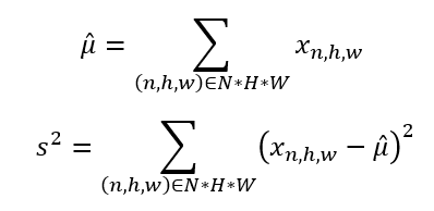
First, we need to calculate batch statistics, in particular, the mean and variance for each of the different activations across a batch. Since each layer’s output serves as an input into the next layer in a neural network, by standardizing the output of the layers, we are also standardizing the inputs to the next layer in our model (though in practice, it was suggested in the original paper to implement batch normalization before the activation function, however there’s some debate over this).

So, we calculate

Then, for each of the activation maps, we normalization each value using the respective statistics

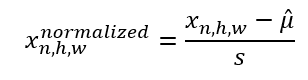
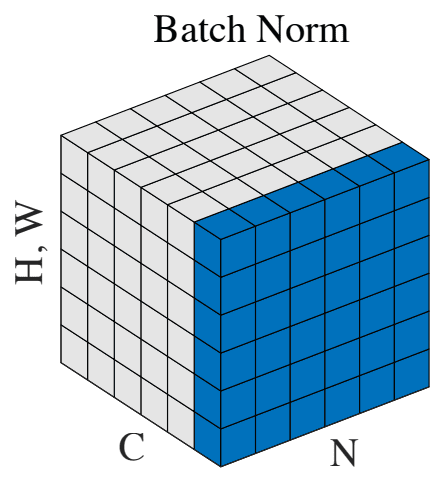
For Convolutional Neural Networks (CNNs) in particular, we calculate these statistics over all locations of the same channel. From the original bath normalization paper,

“For convolutional layers, we additionally want the normalization to obey the convolutional property – so that different elements of the same feature map, at different locations, are normalized in the same way”

Now that we’ve seen how to calculate the normalized activation maps, let’s explore how this can be implemented using Numpy arrays.

Suppose we had these activation maps with all of them representing a single channel,

import numpy as np

activation_map_sample1 = np.array([
[1, 1, 1],
[1, 1, 1],
[1, 1, 1]
], dtype=np.float32)

activation_map_sample2 = np.array([
[1, 2, 3],
[4, 5, 6],
[7, 8, 9]
], dtype=np.float32)

activation_map_sample3 = np.array([
[9, 8, 7],
[6, 5, 4],
[3, 2, 1]
], dtype=np.float32)

Then, we want to standardize each element in the activation map across all locations and across the different samples. To standardize, we compute their mean and standard deviation using

#get mean across the different samples in batch for each activation
activation_mean_bn = np.mean([activation_map_sample1, activation_map_sample2, activation_map_sample3], axis=0)

#get standard deviation across different samples in batch for each activation
activation_std_bn = np.std([activation_map_sample1, activation_map_sample2, activation_map_sample3], axis=0)

print (activation_mean_bn)
print (activation_std_bn)

which outputs

3.6666667
2.8284268

Then, we can standardize an activation map by doing

#get batch normalized activation map for sample 1
activation_map_sample1_bn = (activation_map_sample1 – activation_mean_bn) / activation_std_bn

and these store the outputs

activation_map_sample1_bn:
[[-0.94280916 -0.94280916 -0.94280916]
[-0.94280916 -0.94280916 -0.94280916]
[-0.94280916 -0.94280916 -0.94280916]]

activation_map_sample2_bn:
[[-0.94280916 -0.58925575 -0.2357023 ]
[ 0.11785112 0.47140455 0.82495797]
[ 1.1785114 1.5320647 1.8856182 ]]

activation_map_sample3_bn:
[[ 1.8856182 1.5320647 1.1785114 ]
[ 0.82495797 0.47140455 0.11785112]
[-0.2357023 -0.58925575 -0.94280916]]

But we hit a snag when it comes to inference time. What if we don’t have batches of examples at inference time and even if we did, it would still be preferable if the output is computed from the input deterministically. So, we need to calculate a fixed set of parameters to be used at inference time. For this purpose, we store a moving average for the means and variances instead which we use at inference time to compute the outputs of the layers.

However, another problem with simply standardizing the inputs to a model in this way also changes the representational ability of the layers. One example brought up in the batch normalization paper was the sigmoid nonlinear function, where normalizing the inputs would constrain it to the linear regime of the sigmoid function. To address this, another linear layer is added to scale and recenter the values, along with 2 trainable parameters to learn the appropriate scale and center that should be used.

Implementing Batch Normalization in TensorFlow

Now that we understand what goes on with batch normalization under the hood, let’s see how we can use Keras’ batch normalization layer as part of our deep learning models.

To implement batch normalization as part of our deep learning models in Tensorflow, we can use the keras.layers.BatchNormalization layer. Using the Numpy arrays from our previous example, we can implement the BatchNormalization on them.

import tensorflow as tf
import tensorflow.keras as keras
from tensorflow.keras.layers import BatchNormalization
import numpy as np

#expand dims to create the channels
activation_maps = tf.constant(np.expand_dims(np.stack([activation_map_sample1, activation_map_sample2, activation_map_sample3]), axis=0), dtype=tf.float32)

print (f”activation_maps: n{activation_maps}n”)

print (BatchNormalization(axis=0)(activation_maps, training=True))

which gives us the output

activation_maps:
[[[[1. 1. 1.]
[1. 1. 1.]
[1. 1. 1.]]

[[1. 2. 3.]
[4. 5. 6.]
[7. 8. 9.]]

[[9. 8. 7.]
[6. 5. 4.]
[3. 2. 1.]]]]

tf.Tensor(
[[[[-0.9427501 -0.9427501 -0.9427501 ]
[-0.9427501 -0.9427501 -0.9427501 ]
[-0.9427501 -0.9427501 -0.9427501 ]]

[[-0.9427501 -0.5892188 -0.2356875 ]
[ 0.11784375 0.471375 0.82490635]
[ 1.1784375 1.5319688 1.8855002 ]]

[[ 1.8855002 1.5319688 1.1784375 ]
[ 0.82490635 0.471375 0.11784375]
[-0.2356875 -0.5892188 -0.9427501 ]]]], shape=(1, 3, 3, 3), dtype=float32)

By default, the BatchNormalization layer uses a scale of 1 and center of 0 for the linear layer, hence these values are similar to the values that we computed earlier using Numpy functions.

Normalization and Batch Normalization in Action

Now that we’ve seen how to implement the normalization and batch normalization layers in Tensorflow, let’s explore a LeNet-5 model that uses the normalization and batch normalization layers, as well as compare it to a model that does not use either of these layers.

First, let’s get our dataset, we’ll use CIFAR-10 for this example.

(trainX, trainY), (testX, testY) = keras.datasets.cifar10.load_data()

Using a LeNet-5 model with ReLU activation,

from tensorflow.keras.layers import Dense, Input, Flatten, Conv2D, MaxPool2D
from tensorflow.keras.models import Model
import tensorflow as tf

class LeNet5(tf.keras.Model):
def __init__(self):
super(LeNet5, self).__init__()
def call(self, input_tensor):
self.conv1 = Conv2D(filters=6, kernel_size=(5,5), padding=”same”, activation=”relu”)(input_tensor)
self.maxpool1 = MaxPool2D(pool_size=(2,2))(self.conv1)
self.conv2 = Conv2D(filters=16, kernel_size=(5,5), padding=”same”, activation=”relu”)(self.maxpool1)
self.maxpool2 = MaxPool2D(pool_size=(2, 2))(self.conv2)
self.flatten = Flatten()(self.maxpool2)
self.fc1 = Dense(units=120, activation=”relu”)(self.flatten)
self.fc2 = Dense(units=84, activation=”relu”)(self.fc1)
self.fc3 = Dense(units=10, activation=”sigmoid”)(self.fc2)
return self.fc3

input_layer = Input(shape=(32,32,3,))
x = LeNet5()(input_layer)

model = Model(inputs=input_layer, outputs=x)

model.compile(optimizer=”adam”, loss=tf.keras.losses.SparseCategoricalCrossentropy(), metrics=”acc”)

history = model.fit(x=trainX, y=trainY, batch_size=256, epochs=10, validation_data=(testX, testY))

Training the model gives us the output,

Epoch 1/10
196/196 [==============================] – 14s 15ms/step – loss: 3.8905 – acc: 0.2172 – val_loss: 1.9656 – val_acc: 0.2853
Epoch 2/10
196/196 [==============================] – 2s 12ms/step – loss: 1.8402 – acc: 0.3375 – val_loss: 1.7654 – val_acc: 0.3678
Epoch 3/10
196/196 [==============================] – 2s 12ms/step – loss: 1.6778 – acc: 0.3986 – val_loss: 1.6484 – val_acc: 0.4039
Epoch 4/10
196/196 [==============================] – 2s 12ms/step – loss: 1.5663 – acc: 0.4355 – val_loss: 1.5644 – val_acc: 0.4380
Epoch 5/10
196/196 [==============================] – 2s 12ms/step – loss: 1.4815 – acc: 0.4712 – val_loss: 1.5357 – val_acc: 0.4472
Epoch 6/10
196/196 [==============================] – 2s 12ms/step – loss: 1.4053 – acc: 0.4975 – val_loss: 1.4883 – val_acc: 0.4675
Epoch 7/10
196/196 [==============================] – 2s 12ms/step – loss: 1.3300 – acc: 0.5262 – val_loss: 1.4643 – val_acc: 0.4805
Epoch 8/10
196/196 [==============================] – 2s 12ms/step – loss: 1.2595 – acc: 0.5531 – val_loss: 1.4685 – val_acc: 0.4866
Epoch 9/10
196/196 [==============================] – 2s 12ms/step – loss: 1.1999 – acc: 0.5752 – val_loss: 1.4302 – val_acc: 0.5026
Epoch 10/10
196/196 [==============================] – 2s 12ms/step – loss: 1.1370 – acc: 0.5979 – val_loss: 1.4441 – val_acc: 0.5009

Next, let’s take a look at what happens if we added normalization and batch normalization layers. We usually add layer normalization. Amending our LeNet-5 model,

class LeNet5_Norm(tf.keras.Model):
def __init__(self, norm_layer, *args, **kwargs):
super(LeNet5_Norm, self).__init__()
self.conv1 = Conv2D(filters=6, kernel_size=(5,5), padding=”same”)
self.norm1 = norm_layer(*args, **kwargs)
self.relu = relu
self.max_pool2x2 = MaxPool2D(pool_size=(2,2))
self.conv2 = Conv2D(filters=16, kernel_size=(5,5), padding=”same”)
self.norm2 = norm_layer(*args, **kwargs)
self.flatten = Flatten()
self.fc1 = Dense(units=120)
self.norm3 = norm_layer(*args, **kwargs)
self.fc2 = Dense(units=84)
self.norm4 = norm_layer(*args, **kwargs)
self.fc3 = Dense(units=10, activation=”softmax”)
def call(self, input_tensor):
conv1 = self.conv1(input_tensor)
conv1 = self.norm1(conv1)
conv1 = self.relu(conv1)
maxpool1 = self.max_pool2x2(conv1)
conv2 = self.conv2(maxpool1)
conv2 = self.norm2(conv2)
conv2 = self.relu(conv2)
maxpool2 = self.max_pool2x2(conv2)
flatten = self.flatten(maxpool2)
fc1 = self.fc1(flatten)
fc1 = self.norm3(fc1)
fc1 = self.relu(fc1)
fc2 = self.fc2(fc1)
fc2 = self.norm4(fc2)
fc2 = self.relu(fc2)
fc3 = self.fc3(fc2)
return fc3

And running the training again, this time with the normalization layer added.

normalization_layer = Normalization()
normalization_layer.adapt(trainX)

input_layer = Input(shape=(32,32,3,))
x = LeNet5_Norm(BatchNormalization)(normalization_layer(input_layer))

model = Model(inputs=input_layer, outputs=x)

model.compile(optimizer=”adam”, loss=tf.keras.losses.SparseCategoricalCrossentropy(), metrics=”acc”)

history = model.fit(x=trainX, y=trainY, batch_size=256, epochs=10, validation_data=(testX, testY))

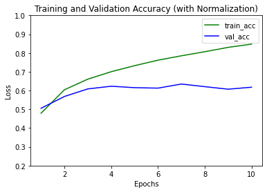
And we see that the model converges faster and gets a higher validation accuracy.

Epoch 1/10
196/196 [==============================] – 5s 17ms/step – loss: 1.4643 – acc: 0.4791 – val_loss: 1.3837 – val_acc: 0.5054
Epoch 2/10
196/196 [==============================] – 3s 14ms/step – loss: 1.1171 – acc: 0.6041 – val_loss: 1.2150 – val_acc: 0.5683
Epoch 3/10
196/196 [==============================] – 3s 14ms/step – loss: 0.9627 – acc: 0.6606 – val_loss: 1.1038 – val_acc: 0.6086
Epoch 4/10
196/196 [==============================] – 3s 14ms/step – loss: 0.8560 – acc: 0.7003 – val_loss: 1.0976 – val_acc: 0.6229
Epoch 5/10
196/196 [==============================] – 3s 14ms/step – loss: 0.7644 – acc: 0.7325 – val_loss: 1.1073 – val_acc: 0.6153
Epoch 6/10
196/196 [==============================] – 3s 15ms/step – loss: 0.6872 – acc: 0.7617 – val_loss: 1.1484 – val_acc: 0.6128
Epoch 7/10
196/196 [==============================] – 3s 14ms/step – loss: 0.6229 – acc: 0.7850 – val_loss: 1.1469 – val_acc: 0.6346
Epoch 8/10
196/196 [==============================] – 3s 14ms/step – loss: 0.5583 – acc: 0.8067 – val_loss: 1.2041 – val_acc: 0.6206
Epoch 9/10
196/196 [==============================] – 3s 15ms/step – loss: 0.4998 – acc: 0.8300 – val_loss: 1.3095 – val_acc: 0.6071
Epoch 10/10
196/196 [==============================] – 3s 14ms/step – loss: 0.4474 – acc: 0.8471 – val_loss: 1.2649 – val_acc: 0.6177

Plotting the train and validation accuracies of both models,

Some caution when using batch normalization, it’s generally not advised to use batch normalization together with dropout as batch normalization has a regularizing effect. Also, too small batch sizes might be an issue for batch normalization as the quality of the statistics (mean and variance) calculated is affected by the batch size and very small batch sizes could lead to issues, with the extreme case being one sample have all activations as 0 if looking at simple neural networks. Consider using layer normalization (more resources in further reading section below) if you are considering using small batch sizes.

Here’s the complete code for the model with normalization too.

from tensorflow.keras.layers import Dense, Input, Flatten, Conv2D, BatchNormalization, MaxPool2D, Normalization
from tensorflow.keras.models import Model
import tensorflow as tf
import tensorflow.keras as keras

class LeNet5_Norm(tf.keras.Model):
def __init__(self, norm_layer, *args, **kwargs):
super(LeNet5_Norm, self).__init__()
self.conv1 = Conv2D(filters=6, kernel_size=(5,5), padding=”same”)
self.norm1 = norm_layer(*args, **kwargs)
self.relu = relu
self.max_pool2x2 = MaxPool2D(pool_size=(2,2))
self.conv2 = Conv2D(filters=16, kernel_size=(5,5), padding=”same”)
self.norm2 = norm_layer(*args, **kwargs)
self.flatten = Flatten()
self.fc1 = Dense(units=120)
self.norm3 = norm_layer(*args, **kwargs)
self.fc2 = Dense(units=84)
self.norm4 = norm_layer(*args, **kwargs)
self.fc3 = Dense(units=10, activation=”softmax”)
def call(self, input_tensor):
conv1 = self.conv1(input_tensor)
conv1 = self.norm1(conv1)
conv1 = self.relu(conv1)
maxpool1 = self.max_pool2x2(conv1)
conv2 = self.conv2(maxpool1)
conv2 = self.norm2(conv2)
conv2 = self.relu(conv2)
maxpool2 = self.max_pool2x2(conv2)
flatten = self.flatten(maxpool2)
fc1 = self.fc1(flatten)
fc1 = self.norm3(fc1)
fc1 = self.relu(fc1)
fc2 = self.fc2(fc1)
fc2 = self.norm4(fc2)
fc2 = self.relu(fc2)
fc3 = self.fc3(fc2)
return fc3

# load dataset, using cifar10 to show greater improvement in accuracy
(trainX, trainY), (testX, testY) = keras.datasets.cifar10.load_data()

normalization_layer = Normalization()
normalization_layer.adapt(trainX)

input_layer = Input(shape=(32,32,3,))
x = LeNet5_Norm(BatchNormalization)(normalization_layer(input_layer))

model = Model(inputs=input_layer, outputs=x)

model.compile(optimizer=”adam”, loss=tf.keras.losses.SparseCategoricalCrossentropy(), metrics=”acc”)

history = model.fit(x=trainX, y=trainY, batch_size=256, epochs=10, validation_data=(testX, testY))

Further Reading

Here are some of the different types of normalization that you can implement in your model:

Layer normalization
Group normalization
Instance Normalization: The Missing Ingredient for Fast Stylization

Tensorflow layers:

Tensorflow addons (Layer, Instance, Group normalization): https://github.com/tensorflow/addons/blob/master/docs/tutorials/layers_normalizations.ipynb
Batch normalization
Normalization

Conclusion

In this post, you’ve discovered how normalization and batch normalization works, as well as how to implement them in TensorFlow. You have also seen how using these layers can help to significantly improve the performance of our machine learning models.

Specifically, you’ve learned:

What normalization and batch normalization does
How to use normalization and batch normalization in TensorFlow
Some tips when using batch normalization in your machine learning model

The post Using Normalization Layers to Improve Deep Learning Models appeared first on Machine Learning Mastery.

Read MoreMachine Learning Mastery