

Last Updated on August 4, 2022
Looking at all of the very large convolutional neural networks such as ResNets, VGGs, and the like, it begs the question on how we can make all of these networks smaller with less parameters while still maintaining the same level of accuracy or even improving generalization of the model using a smaller amount of parameters. One approach is depthwise separable convolutions, also known by separable convolutions in TensorFlow and Pytorch (not to be confused with spatially separable convolutions which are also referred to as separable convolutions). Depthwise separable convolutions were introduced by Sifre in “Rigid-motion scattering for image classification” and has been adopted by popular model architectures such as MobileNet and a similar version in Xception. It splits the channel and spatial convolutions that are usually combined together in normal convolutional layers
In this tutorial, we’ll be looking at what depthwise separable convolutions are and how we can use them to speed up our convolutional neural network image models.
After completing this tutorial, you will learn:
What is a depthwise, pointwise, and depthwise separable convolution
How to implement depthwise separable convolutions in Tensorflow
Using them as part of our computer vision models
Let’s get started!
Using Depthwise Separable Convolutions in Tensorflow
Photo by Arisa Chattasa. Some rights reserved.
Overview
This tutorial is split into 3 parts:
What is a depthwise separable convolution
Why are they useful
Using depthwise separable convolutions in computer vision model
What is a Depthwise Separable Convolution
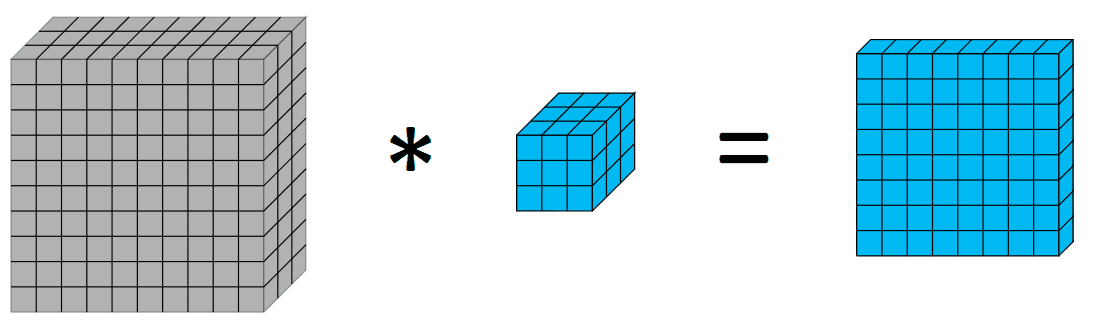
Before diving into depthwise and depthwise separable convolutions, it might be helpful to have a quick recap on convolutions. Convolutions in image processing is a process of applying a kernel over volume, where we do a weighted sum of the pixels with the weights as the values of the kernels. Visually as follows:
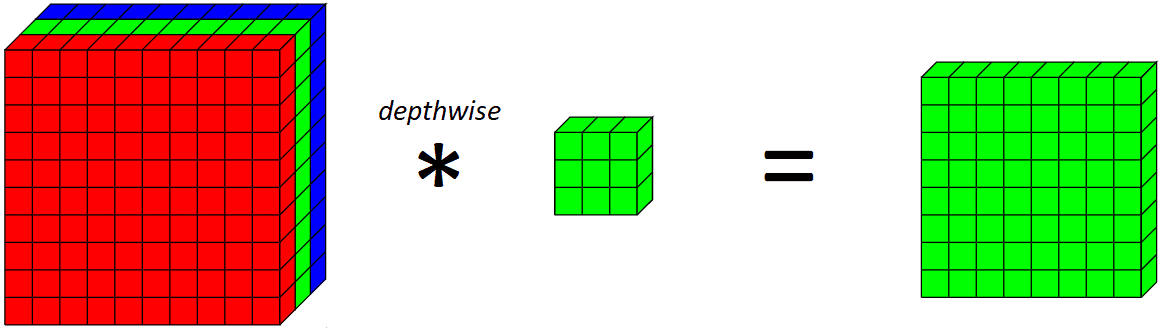
Now, let’s introduce a depthwise convolution. A depthwise convolution is basically a convolution along only one spatial dimension of the image. Visually, this is what a single depthwise convolutional filter would look like and do:
The key difference between a normal convolutional layer and a depthwise convolution is that the depthwise convolution applies the convolution along only one spatial dimension (i.e. channel) while a normal convolution is applied across all spatial dimensions/channels at each step.
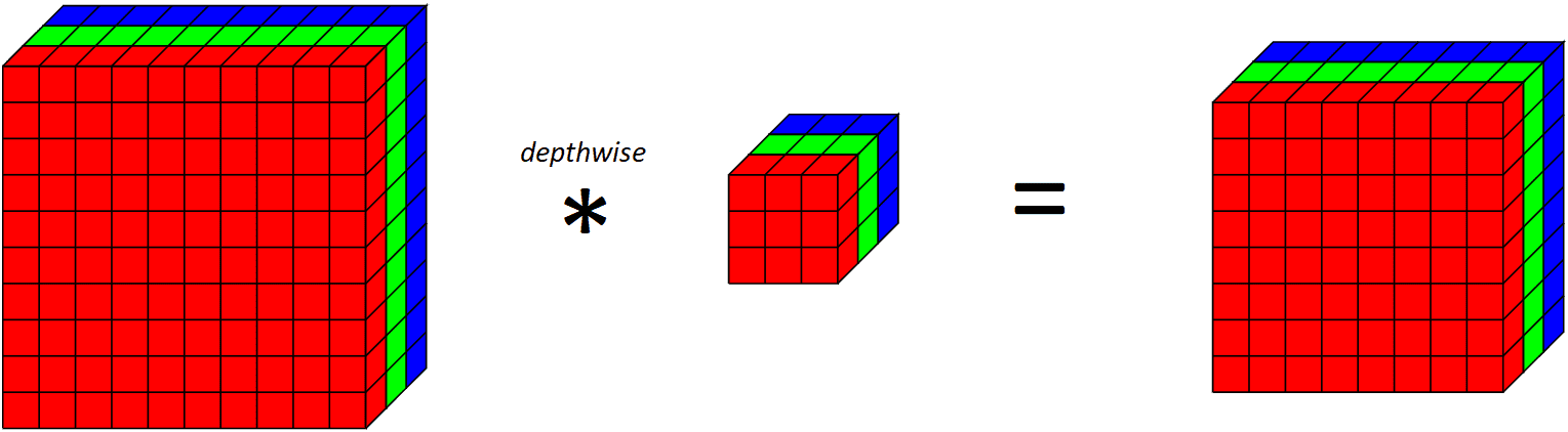
If we look at what an entire depthwise layer does on all RGB channels,
Notice that since we are applying one convolutional filter for each output channel, the number of output channels is equal to the number of input channels. After applying this depthwise convolutional layer, we then apply a pointwise convolutional layer.
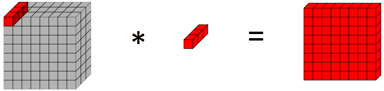
Simply put a pointwise convolutional layer is a regular convolutional layer with a 1×1 kernel (hence looking at a single point across all the channels). Visually, it looks like this:
Why are Depthwise Separable Convolutions Useful?
Now, you might be wondering, what’s the use of doing two operations with the depthwise separable convolutions? Given that the title of this article is to speed up computer vision models, how does doing two operations instead of one help to speed things up?
To answer that question, let’s look at the number of parameters in the model (there would be some additional overhead associated with doing two convolutions instead of one though). Let’s say we wanted to apply 64 convolutional filters to our RGB image to have 64 channels in our output. Number of parameters in normal convolutional layer (including bias term) is $ 3 times 3 times 3 times 64 + 64 = 1792$. On the other hand, using a depthwise separable convolutional layer would only have $(3 times 3 times 1 times 3 + 3) + (1 times 1 times 3 times 64 + 64) = 30 + 256 = 286$ parameters, which is a significant reduction, with depthwise separable convolutions having less than 6 times the parameters of the normal convolution.
This can help to reduce the number of computations and parameters, which reduces training/inference time and can help to regularize our model respectively.
Let’s see this in action. For our inputs, let’s use the CIFAR10 image dataset of 32x32x3 images,
import tensorflow.keras as keras
from keras.datasets import mnist
# load dataset
(trainX, trainY), (testX, testY) = keras.datasets.cifar10.load_data()
Then, we implement a depthwise separable convolution layer. There’s an implementation in Tensorflow but we’ll go into that in the final example.
class DepthwiseSeparableConv2D(keras.layers.Layer):
def __init__(self, filters, kernel_size, padding, activation):
super(DepthwiseSeparableConv2D, self).__init__()
self.depthwise = DepthwiseConv2D(kernel_size = kernel_size, padding = padding, activation = activation)
self.pointwise = Conv2D(filters = filters, kernel_size = (1, 1), activation = activation)
def call(self, input_tensor):
x = self.depthwise(input_tensor)
return self.pointwise(x)
Constructing a model with using a depthwise separable convolutional layer and looking at the number of parameters,
visible = Input(shape=(32, 32, 3))
depthwise_separable = DepthwiseSeparableConv2D(filters=64, kernel_size=(3,3), padding=”valid”, activation=”relu”)(visible)
depthwise_model = Model(inputs=visible, outputs=depthwise_separable)
depthwise_model.summary()
which gives the output
_________________________________________________________________
Layer (type) Output Shape Param #
=================================================================
input_15 (InputLayer) [(None, 32, 32, 3)] 0
depthwise_separable_conv2d_ (None, 30, 30, 64) 286
11 (DepthwiseSeparableConv2
D)
=================================================================
Total params: 286
Trainable params: 286
Non-trainable params: 0
_________________________________________________________________
which we can compare with a similar model using a regular 2D convolutional layer,
normal = Conv2D(filters=64, kernel_size=(3,3), padding=”valid”, activation=”relu”)(visible)
which gives the output
_________________________________________________________________
Layer (type) Output Shape Param #
=================================================================
input (InputLayer) [(None, 32, 32, 3)] 0
conv2d (Conv2D) (None, 30, 30, 64) 1792
=================================================================
Total params: 1,792
Trainable params: 1,792
Non-trainable params: 0
_________________________________________________________________
That corroborates with our initial calculations on the number of parameters done earlier and shows the reduction in number of parameters that can be achieved by using depthwise separable convolutions.
More specifically, let’s look at the number and size of kernels in a normal convolutional layer and a depthwise separable one. When looking at a regular 2D convolutional layer with $c$ channels as inputs, $w times h$ kernel spatial resolution, and $n$ channels as output, we would need to have $(n, w, h, c)$ parameters, that is $n$ filters, with each filter having a kernel size of $(w, h, c)$. However, this is different for a similar depthwise separable convolution even with the same number of input channels, kernel spatial resolution, and output channels. First, there’s the depthwise convolution which involves $c$ filters, each with a kernel size of $(w, h, 1)$ which outputs $c$ channels since it acts on each filter. This depthwise convolutional layer has $(c, w, h, 1)$ parameters (plus some bias units). Then comes the pointwise convolution which takes in the $c$ channels from the depthwise layer, and outputs $n$ channels, so we have $n$ filters each with a kernel size of $(1, 1, n)$. This pointwise convolutional layer has $(n, 1, 1, n)$ parameters (plus some bias units).
You might be thinking right now, but why do they work?
One way of thinking about it, from the Xception paper by Chollet is that depthwise separable convolutions have the assumption that we can separately map cross-channel and spatial correlations. Given this, there will be bunch of redundant weights in the convolutional layer which we can reduce by separating the convolution into two convolutions of the depthwise and pointwise component. One way of thinking about it for those familiar with linear algebra is how we are able to decompose a matrix into outer product of two vectors when the column vectors in the matrix are multiples of each other.
Using Depthwise Separable Convolutions in Computer Vision Models
Now that we’ve seen the reduction in parameters that we can achieve by using a depthwise separable convolution over a normal convolutional filter, let’s see how we can use it in practice with Tensorflow’s SeparableConv2D filter.
For this example, we will be using the CIFAR-10 image dataset used in the above example, while for the model we will be using a model built off VGG blocks. The potential of depthwise separable convolutions is in deeper models where the regularization effect is more beneficial to the model and the reduction in parameters is more obvious as opposed to a lighter weight model such as LeNet-5.
Creating our model using VGG blocks using normal convolutional layers,
from keras.models import Model
from keras.layers import Input, Conv2D, MaxPooling2D, Dense, Flatten, SeparableConv2D
import tensorflow as tf
# function for creating a vgg block
def vgg_block(layer_in, n_filters, n_conv):
# add convolutional layers
for _ in range(n_conv):
layer_in = Conv2D(filters = n_filters, kernel_size = (3,3), padding=’same’, activation=”relu”)(layer_in)
# add max pooling layer
layer_in = MaxPooling2D((2,2), strides=(2,2))(layer_in)
return layer_in
visible = Input(shape=(32, 32, 3))
layer = vgg_block(visible, 64, 2)
layer = vgg_block(layer, 128, 2)
layer = vgg_block(layer, 256, 2)
layer = Flatten()(layer)
layer = Dense(units=10, activation=”softmax”)(layer)
# create model
model = Model(inputs=visible, outputs=layer)
# summarize model
model.summary()
model.compile(optimizer=”adam”, loss=tf.keras.losses.SparseCategoricalCrossentropy(), metrics=”acc”)
history = model.fit(x=trainX, y=trainY, batch_size=128, epochs=10, validation_data=(testX, testY))
Then we look at the results of this 6-layer convolutional neural network with normal convolutional layers,
_________________________________________________________________
Layer (type) Output Shape Param #
=================================================================
input_1 (InputLayer) [(None, 32, 32, 3)] 0
conv2d (Conv2D) (None, 32, 32, 64) 1792
conv2d_1 (Conv2D) (None, 32, 32, 64) 36928
max_pooling2d (MaxPooling2D (None, 16, 16, 64) 0
)
conv2d_2 (Conv2D) (None, 16, 16, 128) 73856
conv2d_3 (Conv2D) (None, 16, 16, 128) 147584
max_pooling2d_1 (MaxPooling (None, 8, 8, 128) 0
2D)
conv2d_4 (Conv2D) (None, 8, 8, 256) 295168
conv2d_5 (Conv2D) (None, 8, 8, 256) 590080
max_pooling2d_2 (MaxPooling (None, 4, 4, 256) 0
2D)
flatten (Flatten) (None, 4096) 0
dense (Dense) (None, 10) 40970
=================================================================
Total params: 1,186,378
Trainable params: 1,186,378
Non-trainable params: 0
_________________________________________________________________
Epoch 1/10
391/391 [==============================] – 11s 27ms/step – loss: 1.7468 – acc: 0.4496 – val_loss: 1.3347 – val_acc: 0.5297
Epoch 2/10
391/391 [==============================] – 10s 26ms/step – loss: 1.0224 – acc: 0.6399 – val_loss: 0.9457 – val_acc: 0.6717
Epoch 3/10
391/391 [==============================] – 10s 26ms/step – loss: 0.7846 – acc: 0.7282 – val_loss: 0.8566 – val_acc: 0.7109
Epoch 4/10
391/391 [==============================] – 10s 26ms/step – loss: 0.6394 – acc: 0.7784 – val_loss: 0.8289 – val_acc: 0.7235
Epoch 5/10
391/391 [==============================] – 10s 26ms/step – loss: 0.5385 – acc: 0.8118 – val_loss: 0.7445 – val_acc: 0.7516
Epoch 6/10
391/391 [==============================] – 11s 27ms/step – loss: 0.4441 – acc: 0.8461 – val_loss: 0.7927 – val_acc: 0.7501
Epoch 7/10
391/391 [==============================] – 11s 27ms/step – loss: 0.3786 – acc: 0.8672 – val_loss: 0.8279 – val_acc: 0.7455
Epoch 8/10
391/391 [==============================] – 10s 26ms/step – loss: 0.3261 – acc: 0.8855 – val_loss: 0.8886 – val_acc: 0.7560
Epoch 9/10
391/391 [==============================] – 10s 27ms/step – loss: 0.2747 – acc: 0.9044 – val_loss: 1.0134 – val_acc: 0.7387
Epoch 10/10
391/391 [==============================] – 10s 26ms/step – loss: 0.2519 – acc: 0.9126 – val_loss: 0.9571 – val_acc: 0.7484
Let’s try out the same architecture but replace the normal convolutional layers with Keras’ SeparableConv2D layers instead:
# depthwise separable VGG block
def vgg_depthwise_block(layer_in, n_filters, n_conv):
# add convolutional layers
for _ in range(n_conv):
layer_in = SeparableConv2D(filters = n_filters, kernel_size = (3,3), padding=’same’, activation=’relu’)(layer_in)
# add max pooling layer
layer_in = MaxPooling2D((2,2), strides=(2,2))(layer_in)
return layer_in
visible = Input(shape=(32, 32, 3))
layer = vgg_depthwise_block(visible, 64, 2)
layer = vgg_depthwise_block(layer, 128, 2)
layer = vgg_depthwise_block(layer, 256, 2)
layer = Flatten()(layer)
layer = Dense(units=10, activation=”softmax”)(layer)
# create model
model = Model(inputs=visible, outputs=layer)
# summarize model
model.summary()
model.compile(optimizer=”adam”, loss=tf.keras.losses.SparseCategoricalCrossentropy(), metrics=”acc”)
history_dsconv = model.fit(x=trainX, y=trainY, batch_size=128, epochs=10, validation_data=(testX, testY))
Running the above code gives us the result:
_________________________________________________________________
Layer (type) Output Shape Param #
=================================================================
input_1 (InputLayer) [(None, 32, 32, 3)] 0
separable_conv2d (Separab (None, 32, 32, 64) 283
leConv2D)
separable_conv2d_2 (Separab (None, 32, 32, 64) 4736
leConv2D)
max_pooling2d (MaxPoolin (None, 16, 16, 64) 0
g2D)
separable_conv2d_3 (Separab (None, 16, 16, 128) 8896
leConv2D)
separable_conv2d_4 (Separab (None, 16, 16, 128) 17664
leConv2D)
max_pooling2d_2 (MaxPoolin (None, 8, 8, 128) 0
g2D)
separable_conv2d_5 (Separa (None, 8, 8, 256) 34176
bleConv2D)
separable_conv2d_6 (Separa (None, 8, 8, 256) 68096
bleConv2D)
max_pooling2d_3 (MaxPoolin (None, 4, 4, 256) 0
g2D)
flatten (Flatten) (None, 4096) 0
dense (Dense) (None, 10) 40970
=================================================================
Total params: 174,821
Trainable params: 174,821
Non-trainable params: 0
_________________________________________________________________
Epoch 1/10
391/391 [==============================] – 10s 22ms/step – loss: 1.7578 – acc: 0.3534 – val_loss: 1.4138 – val_acc: 0.4918
Epoch 2/10
391/391 [==============================] – 8s 21ms/step – loss: 1.2712 – acc: 0.5452 – val_loss: 1.1618 – val_acc: 0.5861
Epoch 3/10
391/391 [==============================] – 8s 22ms/step – loss: 1.0560 – acc: 0.6286 – val_loss: 0.9950 – val_acc: 0.6501
Epoch 4/10
391/391 [==============================] – 8s 21ms/step – loss: 0.9175 – acc: 0.6800 – val_loss: 0.9327 – val_acc: 0.6721
Epoch 5/10
391/391 [==============================] – 9s 22ms/step – loss: 0.7939 – acc: 0.7227 – val_loss: 0.8348 – val_acc: 0.7056
Epoch 6/10
391/391 [==============================] – 8s 22ms/step – loss: 0.7120 – acc: 0.7515 – val_loss: 0.8228 – val_acc: 0.7153
Epoch 7/10
391/391 [==============================] – 8s 21ms/step – loss: 0.6346 – acc: 0.7772 – val_loss: 0.7444 – val_acc: 0.7415
Epoch 8/10
391/391 [==============================] – 8s 21ms/step – loss: 0.5534 – acc: 0.8061 – val_loss: 0.7417 – val_acc: 0.7537
Epoch 9/10
391/391 [==============================] – 8s 21ms/step – loss: 0.4865 – acc: 0.8301 – val_loss: 0.7348 – val_acc: 0.7582
Epoch 10/10
391/391 [==============================] – 8s 21ms/step – loss: 0.4321 – acc: 0.8485 – val_loss: 0.7968 – val_acc: 0.7458
Notice that there are significantly less parameters in the depthwise separable convolution version (~200k vs ~1.2m parameters), along with a slightly lower train time per epoch. Depthwise separable convolutions is more likely to work better on deeper models that might face an overfitting problem and on layers with larger kernels since there is a greater decrease in parameters and computations that would offset the additional computational cost of doing two convolutions instead of one. Next, we plot the train and validation and accuracy of the two models, to see differences in the training performance of the models:
Training and validation accuracy of network with depthwise separable convolutional layers
The highest validation accuracy is similar for both models, but the depthwise separable convolution appears to have less overfitting to the train set, which might help it generalize better to new data.
Combining all the code together for the depthwise separable convolutions version of the model,
import tensorflow.keras as keras
from keras.datasets import mnist
# load dataset
(trainX, trainY), (testX, testY) = keras.datasets.cifar10.load_data()
# depthwise separable VGG block
def vgg_depthwise_block(layer_in, n_filters, n_conv):
# add convolutional layers
for _ in range(n_conv):
layer_in = SeparableConv2D(filters = n_filters, kernel_size = (3,3), padding=’same’,activation=’relu’)(layer_in)
# add max pooling layer
layer_in = MaxPooling2D((2,2), strides=(2,2))(layer_in)
return layer_in
visible = Input(shape=(32, 32, 3))
layer = vgg_depthwise_block(visible, 64, 2)
layer = vgg_depthwise_block(layer, 128, 2)
layer = vgg_depthwise_block(layer, 256, 2)
layer = Flatten()(layer)
layer = Dense(units=10, activation=”softmax”)(layer)
# create model
model = Model(inputs=visible, outputs=layer)
# summarize model
model.summary()
model.compile(optimizer=”adam”, loss=tf.keras.losses.SparseCategoricalCrossentropy(), metrics=”acc”)
history_dsconv = model.fit(x=trainX, y=trainY, batch_size=128, epochs=10, validation_data=(testX, testY))
Further Reading
This section provides more resources on the topic if you are looking to go deeper.
Papers:
Rigid-Motion Scattering For Image Classification (depthwise separable convolutions)
MobileNet
Xception
APIs:
Depthwise Separable Convolutions in Tensorflow (SeparableConv2D)
Summary
In this post, you’ve seen what are depthwise, pointwise, and depthwise separable convolutions. You’ve also seen how using depthwise separable convolutions allows us to get competitive results while using a significantly smaller number of parameters.
Specifically, you’ve learnt:
What is a depthwise, pointwise, and depthwise separable convolution
How to implement depthwise separable convolutions in Tensorflow
Using them as part of our computer vision models
The post Using Depthwise Separable Convolutions in Tensorflow appeared first on Machine Learning Mastery.
Read MoreMachine Learning Mastery