

Amazon DynamoDB is a fully managed and serverless NoSQL cloud database service that provides consistent performance at any scale, with zero-downtime for maintenance or scaling. While there is a maximum item size of 400 KB (inclusive of both attribute names and values), you can use a technique called vertical partitioning to scale your data beyond this limit. For context, in DynamoDB, an item is the equivalent of an individual row and an attribute would be the equivalent of a column in a relational database. There is a correlation between the item size and the cost of read and write operations.
In this post, we discuss reasons to consider vertical partitioning, and how it can be applied in some example scenarios to optimize for throughput and cost. We use the NoSQL Workbench for DynamoDB to model the data and visualize sample records. To download and install NoSQL Workbench for Amazon DynamoDB, see Download NoSQL Workbench.
Data modeling decisions
In DynamoDB, there is no concept of computed table JOINS at the server, and customers often denormalize data in their tables and secondary indexes to optimize for reading. This results in having the same attribute name and value across multiple items. The practice of updating or deleting this data, however, warrants a discussion on integrity and is often application specific, so isn’t covered in this post.
When modeling in this fashion, it’s natural to first consider creating a single item (or large document) with all necessary attributes stored inside. This can be effective if the resulting items are small. However, as the item sizes increases, throughput might become less efficient and cost might increase because DynamoDB meters consumption by item size. Also, you might become constrained by the 400 KB item size limit.
Let’s say you have a users table that contains basic user profiles and additional metadata such as their address, shopping cart items, and website display preferences. It would be trivial to dynamically add this information to a single user item as and when necessary. Because DynamoDB is flexible regarding schema, each item can have differing attributes. But what happens if a user adds many shopping cart items and reaches the 400 KB limit? Or you begin to store a lot more data than you had originally planned? In these scenarios, you might not be able to store all the information you need for each item. Worst case, this could lead to application or functionality failure. You might even have to limit the amount of user data you store. Neither of these outcomes are ideal and they can be avoided.
The data model example shown in Figure 1 that follows has one (simplified) item per user. Each item has a randomized, unique internal ID as the partition key value.
Aside from the maximum item size limit, this approach isn’t always optimal. For example, any time you need to update a user item, you’re going to pay the cost for writing the full item back into the table. If that item has 150 KB of data and you want to change one attribute, let’s say a user’s email address, it’s going to consume 150 write capacity units (WCU). When you read a user item into your application to work with their email address, you have to read the whole item from DynamoDB. With a 150 KB item size, this is going to consume 37.5 read capacity units (RCU) when using the default eventually consistent reads. The same principle applies if the item is 250 KB or 350 KB. As you can see, this is neither optimal nor efficient for your application.
An introduction to vertical partitioning
The solution to the large item quandary is to break items down into smaller chunks of data, associating all relevant items by the partition key value. You can then use a sort key string to identify the associated information stored alongside it. By doing this, and having multiple items grouped by the same partition key value, you are creating an item collection.
Let’s see how this looks in practice in Figure 2 that follows:
Figure 2 shows that, by creating an item collection, we now have multiple items (seven to be exact) with each item grouped by the partition key value. We’re using the sort key to distribute and identify the user item in smaller logical chunks of data. We also added some additional items of data to illustrate a larger item collection. This demonstrates how DynamoDB allows you to effectively have a different schema per item, unlike relational databases, attributes (or columns) don’t always have to be used, or be the same for each item.
The sort key naming convention you choose is up to you, but it’s recommended to keep it short and meaningful. In this example, we use a prefix of U# to specify core user information, M# to specify additional metadata, and P# to call out preference information. It’s also recommended to use the most common identifiers at the start of the string, and the more unique towards the end—we’ll cover why this is important shortly.
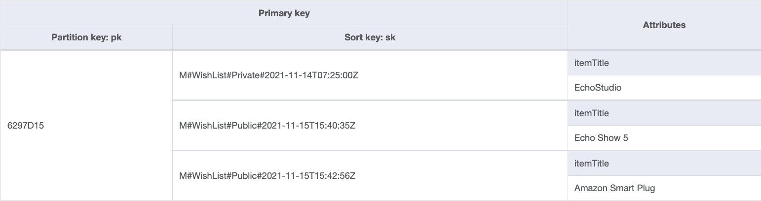
By splitting the data into smaller items, you can perform highly targeted queries against data stored in DynamoDB. This method also future proofs your data storage needs. Let’s say you need to add a new group of data for a user—for example, your organization decides to implement a Wish List system into the platform six months after launch. You can create a new item for that user (partition key: 6297D15) and use the sort key prefix value (M#WishList#Public or M#WishList#Private) to describe and store the new information. This is a fundamental principle for scaling out data within DynamoDB.
In the preceding Figure 3, there are three items stored across the user’s Wish Lists. We also appended a timestamp to the end of the sort key attribute, the reason for this is twofold.
First, when working on the base table (and not in a global secondary index (GSI)), the primary key value (partition key and sort key) must be unique. Because the user in this example has two items in their public Wish List, we can’t use M#WishList#Public twice because it wouldn’t be unique. Appending a timestamp helps to create a distinct value (the timestamp formatting and level are at your discretion).
Second, it helps by acting as a natural sorting mechanism when pulling results from any Wish List queries. When you run a query against DynamoDB, the results you receive are always sorted by the sort key value. If the data type of the sort key is Number, the results are returned in numeric order. Otherwise, the results are returned in order of UTF-8 bytes. By default, the sort order is ascending. If you were to query all the items for the user (where the partition key value is 6297D15) on their public Wish List (where the sort key begins with M#WishList#Public), the results would be returned in chronological order, with the oldest items returned first. To reverse the order, set the ScanIndexForward parameter of the query to false.
Whether you’re performing a GetItem or a query with DynamoDB, you must know at least the partition key value. Without this information you cannot get your items back without performing non-optimized operations such as a Scan. When you have the partition key value, you don’t always need to know the values of your sort keys. With that, how do you know how to retrieve data scoped by a user, or how do you retrieve or update (or even delete) only specific items? The answer lies in sort key targeting.
Performing highly targeted queries
By using the sort key to provide meaningful context to the item (and the attributes associated with it), you can use queries to target specific items or groups of items within the item collection. We mentioned earlier that it’s recommended to use the most common keyword at the start of the sort key value, followed by the least common to the right. What’s the value in doing that? Let’s look at some examples written in Python using the boto3 SDK.
If you want to get back all items associated to a user (6297D15), you can call:
The results of this query contain the entire item collection: Preferences (P#), user information (U#), and metadata (M#) for all 10 user items (now that we have added three Wish List items). While that could be useful, it’s no more efficient than storing a large item to begin with—something we’re trying to avoid. Let’s say you only want the user information (U#) from the collection for a given user; that’s done by using the begins_with operator to specify that the key condition expression matches values that begin with U#:
Figure 4 that follows shows the results of this query. It only returns the user information items U#Address#Delivery, U#Address#Home, and U#Information.
The begins_with operator narrows down the matching items from the table that are returned based on the sort key value (matching from left-to-right). For example, if you’re only interested in the Address information, you can tell DynamoDB to return only those matching items by narrowing down the string-matching as follows:
Now the query results will only contain the U#Address items. DynamoDB has discarded the other item (U#Information) as it doesn’t fulfil the string-matching criteria, and you avoided a charge for RCUs to retrieve unwanted data from the table. If you know the sort key value in its entirety and need to retrieve only that item, you don’t need to use begins_with but can match using the equals operator:
With the understanding of how to use begins_with, let’s revisit the Wish List items from the collection.
Wish lists revisited
Earlier, we discussed using a timestamp for both uniqueness and for sorting results when performing a query. To get all Wish List items for a given user, regardless of whether it’s on their Public or Private list, you can use the following query:
The example above will return the results sorted by UTF-8 character code values. You get the Private Wish List item first, followed by the Public Wish List items, ordered by the oldest items first. If you want to get items that belong to specific list, you can use the following query:
An additional benefit to using a timestamp in this manner is that it allows you to further refine your Wish List queries. Let’s say you wanted to get all items from the public list that were added in 2021, or better yet, were added in November of 2021—begins_with makes this level of targeting possible:
You should now be able to see the power that combining vertical partitioning with the query capabilities of DynamoDB gives you to isolate specific items inside your item collection. You can return single items or multiple items by harnessing commonalities in the matching pattern, through to returning specific items by decreasing the matching scope.
What about initial and ongoing costs?
We’ve covered how breaking down a large item into smaller ones and using sort keys to define context and the relationship of the corresponding data lets you ask DynamoDB to return just the exact items you require. You no longer have to pull down an entire item just to read 1 KB (or less) of data. Remember that hypothetical 150 KB item? Instead of it costing 37.5 RCUs to read in the users email address, it now costs just 0.5 RCU. Similarly, you no longer have to pay the cost of writing the entire item back just to update a user’s name or email value, or add an item to their Wish List. This is where the power of vertical partitioning has a direct impact on the overall cost of running and maintaining your data in DynamoDB.
But what about writing the initial item and all the data to begin with, how does the cost change here? It’s important to note that if you’re building your data up over time, there would be no change to ongoing costs compared to the first item write. However, if you’re taking an existing large item and breaking it down into this format, there might be an initial increase of cost to rewrite the item data out—let’s discuss that in more detail.
Depending on how the item is broken down (let’s say it consists of 100 key-value pairs), writing this into DynamoDB in a vertically partitioned model could consume more write units for the initial write. Why so? Well, a write unit is charged on a per 1 KB unit and is rounded up, so if you’re writing 125 bytes of data, you would be charged 1 WCU for each write. If you’re writing 100 items (each item is under 1 KB) you’re going to be charged 100 WCUs (100 x (1 KB @ 1 unit) = 100 WCUs). If you stored all the key pairs as one large object, then DynamoDB would round up the write. Let’s say in this instance 100 pairs equates to 50 KB of data. In that case, a single initial write in a non-partitioned model would cost 50 WCUs.
You might be thinking, why should I take a write-cost tradeoff with vertical partitioning? Well, in reality, despite the potential first write cost increase, you will break even on write costs after your next update. Again, let’s say you’re updating a user’s email address—updating a large item costs another 50 WCUs (your overall cost so far is now 100 WCUs, increasing 50 WCUs on each update), but with a partitioned model, it only costs 1 WCU per update, so the total cost is now 101 WCUs. Vertical partitioning is more cost efficient from that point on.
Summary
In this post, we discussed the 400 KB item size limit in DynamoDB, how that can prevent large documents of associated data from being stored, and how it can lead to an under-optimized table in terms of cost, throughput, and performance efficiency.
We showed you how you can use vertical partitioning to scale down the data into item collections and how you can use targeted queries to retrieve specific items from a collection, helping increase efficiency while also reducing associated costs.
We hope you’ve found this post useful as a catalyst to revisit how you’re storing data in DynamoDB to see how you can apply this technique to your tables; we’re excited to see what you can do. To learn more about some different options for handling large objects within DynamoDB, see Large object storage strategies for Amazon DynamoDB.
About the authors
Mike Mackay was a Sr. NoSQL Specialist Solutions Architect based in UK.
Samaneh Utter is a Sr. DynamoDB Specialist Solutions Architect based in Göteborg, Sweden.
Read MoreAWS Database Blog