Understanding Simple Recurrent Neural Networks In Keras

Last Updated on September 20, 2022

This tutorial is designed for anyone looking for an understanding of how recurrent neural networks (RNN) work and how to use them via the Keras deep learning library. While all the methods required for solving problems and building applications are provided by the Keras library, it is also important to gain an insight on how everything works. In this article, the computations taking place in the RNN model are shown step by step. Next, a complete end to end system for time series prediction is developed.

After completing this tutorial, you will know:

The structure of RNN
How RNN computes the output when given an input
How to prepare data for a SimpleRNN in Keras
How to train a SimpleRNN model

Let’s get started.

Tutorial Overview

This tutorial is divided into two parts; they are:

The structure of the RNN
Different weights and biases associated with different layers of the RNN.
How computations are performed to compute the output when given an input.

A complete application for time series prediction.

Prerequisites

It is assumed that you have a basic understanding of RNNs before you start implementing them. An Introduction To Recurrent Neural Networks And The Math That Powers Them gives you a quick overview of RNNs.

Let’s now get right down to the implementation part.

Import section

To start the implementation of RNNs, let’s add the import section.

from pandas import read_csv
import numpy as np
from keras.models import Sequential
from keras.layers import Dense, SimpleRNN
from sklearn.preprocessing import MinMaxScaler
from sklearn.metrics import mean_squared_error
import math
import matplotlib.pyplot as plt

Keras SimpleRNN

The function below returns a model that includes a SimpleRNN layer and a Dense layer for learning sequential data. The input_shape specifies the parameter (time_steps x features). We’ll simplify everything and use univariate data, i.e., one feature only; the time_steps are discussed below.

def create_RNN(hidden_units, dense_units, input_shape, activation):
model = Sequential()
model.add(SimpleRNN(hidden_units, input_shape=input_shape,
activation=activation[0]))
model.add(Dense(units=dense_units, activation=activation[1]))
model.compile(loss=’mean_squared_error’, optimizer=’adam’)
return model

demo_model = create_RNN(2, 1, (3,1), activation=[‘linear’, ‘linear’])

The object demo_model is returned with 2 hidden units created via a the SimpleRNN layer and 1 dense unit created via the Dense layer. The input_shape is set at 3×1 and a linear activation function is used in both layers for simplicity. Just to recall the linear activation function $f(x) = x$ makes no change in the input. The network looks as follows:

If we have $m$ hidden units ($m=2$ in the above case), then:

Input: $x in R$
Hidden unit: $h in R^m$
Weights for input units: $w_x in R^m$
Weights for hidden units: $w_h in R^{mxm}$
Bias for hidden units: $b_h in R^m$
Weight for the dense layer: $w_y in R^m$
Bias for the dense layer: $b_y in R$

Let’s look at the above weights. Note: As the weights are initialized randomly, the results pasted here will be different from yours. The important thing is to learn what the structure of each object being used looks like and how it interacts with others to produce the final output.

wx = demo_model.get_weights()[0]
wh = demo_model.get_weights()[1]
bh = demo_model.get_weights()[2]
wy = demo_model.get_weights()[3]
by = demo_model.get_weights()[4]

print(‘wx = ‘, wx, ‘ wh = ‘, wh, ‘ bh = ‘, bh, ‘ wy =’, wy, ‘by = ‘, by)

wx = [[ 0.18662322 -1.2369459 ]] wh = [[ 0.86981213 -0.49338293]
[ 0.49338293 0.8698122 ]] bh = [0. 0.] wy = [[-0.4635998]
[ 0.6538409]] by = [0.]

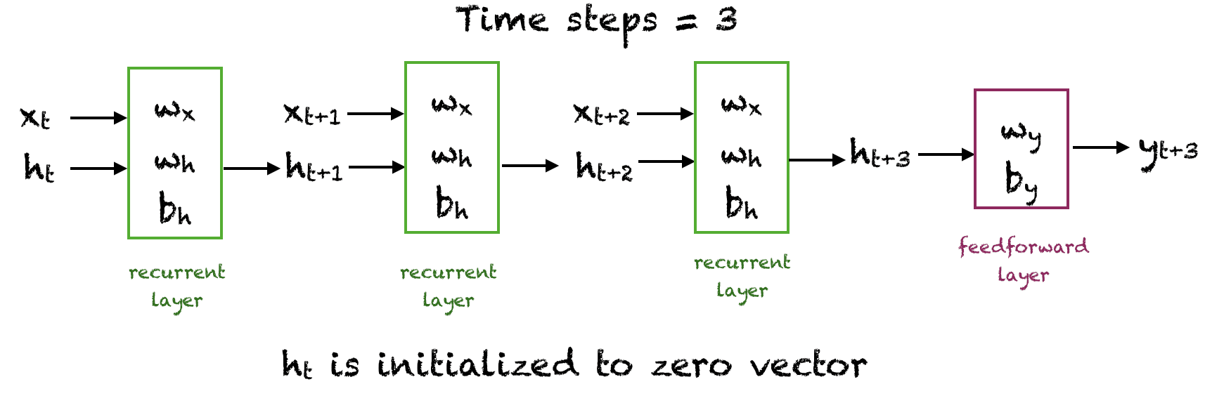
Now let’s do a simple experiment to see how the layers from a SimpleRNN and Dense layer produce an output. Keep this figure in view.

We’ll input x for three time steps and let the network generate an output. The values of the hidden units at time steps 1, 2 and 3 will be computed. $h_0$ is initialized to the zero vector. The output $o_3$ is computed from $h_3$ and $w_y$. An activation function is not required as we are using linear units.

x = np.array([1, 2, 3])
# Reshape the input to the required sample_size x time_steps x features
x_input = np.reshape(x,(1, 3, 1))
y_pred_model = demo_model.predict(x_input)

m = 2
h0 = np.zeros(m)
h1 = np.dot(x[0], wx) + h0 + bh
h2 = np.dot(x[1], wx) + np.dot(h1,wh) + bh
h3 = np.dot(x[2], wx) + np.dot(h2,wh) + bh
o3 = np.dot(h3, wy) + by

print(‘h1 = ‘, h1,’h2 = ‘, h2,’h3 = ‘, h3)

print(“Prediction from network “, y_pred_model)
print(“Prediction from our computation “, o3)

h1 = [[ 0.18662322 -1.23694587]] h2 = [[-0.07471441 -3.64187904]] h3 = [[-1.30195881 -6.84172557]]
Prediction from network [[-3.8698118]]
Prediction from our computation [[-3.86981216]]

Running The RNN On Sunspots Dataset

Now that we understand how the SimpleRNN and Dense layers are put together. Let’s run a complete RNN on a simple time series dataset. We’ll need to follow these steps

Read the dataset from a given URL
Split the data into training and test set
Prepare the input to the required Keras format
Create an RNN model and train it
Make the predictions on training and test sets and print the root mean square error on both sets
View the result

Step 1, 2: Reading Data and Splitting Into Train And Test

The following function reads the train and test data from a given URL and splits it into a given percentage of train and test data. It returns single dimensional arrays for train and test data after scaling the data between 0 and 1 using MinMaxScaler from scikit-learn.

# Parameter split_percent defines the ratio of training examples
def get_train_test(url, split_percent=0.8):
df = read_csv(url, usecols=[1], engine=’python’)
data = np.array(df.values.astype(‘float32’))
scaler = MinMaxScaler(feature_range=(0, 1))
data = scaler.fit_transform(data).flatten()
n = len(data)
# Point for splitting data into train and test
split = int(n*split_percent)
train_data = data[range(split)]
test_data = data[split:]
return train_data, test_data, data

sunspots_url = ‘https://raw.githubusercontent.com/jbrownlee/Datasets/master/monthly-sunspots.csv’
train_data, test_data, data = get_train_test(sunspots_url)

Step 3: Reshaping Data For Keras

The next step is to prepare the data for Keras model training. The input array should be shaped as: total_samples x time_steps x features.

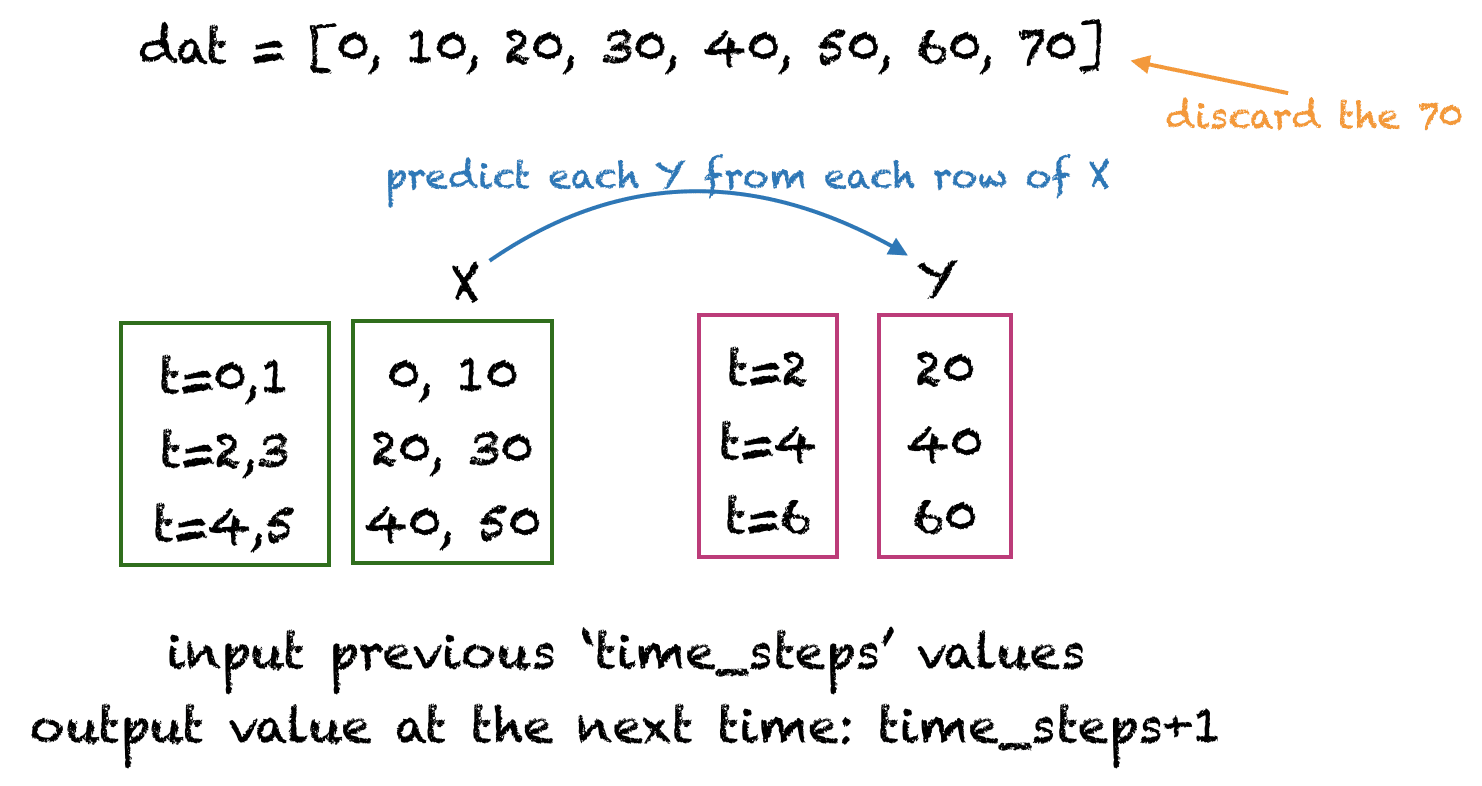
There are many ways of preparing time series data for training. We’ll create input rows with non-overlapping time steps. An example for time_steps = 2 is shown in the figure below. Here time_steps denotes the number of previous time steps to use for predicting the next value of the time series data.

The following function get_XY() takes a one dimensional array as input and converts it to the required input X and target Y arrays. We’ll use 12 time_steps for the sunspots dataset as the sunspots generally have a cycle of 12 months. You can experiment with other values of time_steps.

# Prepare the input X and target Y
def get_XY(dat, time_steps):
# Indices of target array
Y_ind = np.arange(time_steps, len(dat), time_steps)
Y = dat[Y_ind]
# Prepare X
rows_x = len(Y)
X = dat[range(time_steps*rows_x)]
X = np.reshape(X, (rows_x, time_steps, 1))
return X, Y

time_steps = 12
trainX, trainY = get_XY(train_data, time_steps)
testX, testY = get_XY(test_data, time_steps)

Step 4: Create RNN Model And Train

For this step, we can reuse our create_RNN() function that was defined above.

model = create_RNN(hidden_units=3, dense_units=1, input_shape=(time_steps,1),
activation=[‘tanh’, ‘tanh’])
model.fit(trainX, trainY, epochs=20, batch_size=1, verbose=2)

Step 5: Compute And Print The Root Mean Square Error

The function print_error() computes the mean square error between the actual values and the predicted values.

def print_error(trainY, testY, train_predict, test_predict):
# Error of predictions
train_rmse = math.sqrt(mean_squared_error(trainY, train_predict))
test_rmse = math.sqrt(mean_squared_error(testY, test_predict))
# Print RMSE
print(‘Train RMSE: %.3f RMSE’ % (train_rmse))
print(‘Test RMSE: %.3f RMSE’ % (test_rmse))

# make predictions
train_predict = model.predict(trainX)
test_predict = model.predict(testX)
# Mean square error
print_error(trainY, testY, train_predict, test_predict)

Train RMSE: 0.058 RMSE
Test RMSE: 0.077 RMSE

Step 6: View The result

The following function plots the actual target values and the predicted value. The red line separates the training and test data points.

# Plot the result
def plot_result(trainY, testY, train_predict, test_predict):
actual = np.append(trainY, testY)
predictions = np.append(train_predict, test_predict)
rows = len(actual)
plt.figure(figsize=(15, 6), dpi=80)
plt.plot(range(rows), actual)
plt.plot(range(rows), predictions)
plt.axvline(x=len(trainY), color=’r’)
plt.legend([‘Actual’, ‘Predictions’])
plt.xlabel(‘Observation number after given time steps’)
plt.ylabel(‘Sunspots scaled’)
plt.title(‘Actual and Predicted Values. The Red Line Separates The Training And Test Examples’)
plot_result(trainY, testY, train_predict, test_predict)

The following plot is generated:

Consolidated Code

Given below is the entire code for this tutorial. Do try this out at your end and experiment with different hidden units and time steps. You can add a second SimpleRNN to the network and see how it behaves. You can also use the scaler object to rescale the data back to its normal range.

# Parameter split_percent defines the ratio of training examples
def get_train_test(url, split_percent=0.8):
df = read_csv(url, usecols=[1], engine=’python’)
data = np.array(df.values.astype(‘float32’))
scaler = MinMaxScaler(feature_range=(0, 1))
data = scaler.fit_transform(data).flatten()
n = len(data)
# Point for splitting data into train and test
split = int(n*split_percent)
train_data = data[range(split)]
test_data = data[split:]
return train_data, test_data, data

# Prepare the input X and target Y
def get_XY(dat, time_steps):
Y_ind = np.arange(time_steps, len(dat), time_steps)
Y = dat[Y_ind]
rows_x = len(Y)
X = dat[range(time_steps*rows_x)]
X = np.reshape(X, (rows_x, time_steps, 1))
return X, Y

def create_RNN(hidden_units, dense_units, input_shape, activation):
model = Sequential()
model.add(SimpleRNN(hidden_units, input_shape=input_shape, activation=activation[0]))
model.add(Dense(units=dense_units, activation=activation[1]))
model.compile(loss=’mean_squared_error’, optimizer=’adam’)
return model

def print_error(trainY, testY, train_predict, test_predict):
# Error of predictions
train_rmse = math.sqrt(mean_squared_error(trainY, train_predict))
test_rmse = math.sqrt(mean_squared_error(testY, test_predict))
# Print RMSE
print(‘Train RMSE: %.3f RMSE’ % (train_rmse))
print(‘Test RMSE: %.3f RMSE’ % (test_rmse))

# Plot the result
def plot_result(trainY, testY, train_predict, test_predict):
actual = np.append(trainY, testY)
predictions = np.append(train_predict, test_predict)
rows = len(actual)
plt.figure(figsize=(15, 6), dpi=80)
plt.plot(range(rows), actual)
plt.plot(range(rows), predictions)
plt.axvline(x=len(trainY), color=’r’)
plt.legend([‘Actual’, ‘Predictions’])
plt.xlabel(‘Observation number after given time steps’)
plt.ylabel(‘Sunspots scaled’)
plt.title(‘Actual and Predicted Values. The Red Line Separates The Training And Test Examples’)

sunspots_url = ‘https://raw.githubusercontent.com/jbrownlee/Datasets/master/monthly-sunspots.csv’
time_steps = 12
train_data, test_data, data = get_train_test(sunspots_url)
trainX, trainY = get_XY(train_data, time_steps)
testX, testY = get_XY(test_data, time_steps)

# Create model and train
model = create_RNN(hidden_units=3, dense_units=1, input_shape=(time_steps,1),
activation=[‘tanh’, ‘tanh’])
model.fit(trainX, trainY, epochs=20, batch_size=1, verbose=2)

# make predictions
train_predict = model.predict(trainX)
test_predict = model.predict(testX)

# Print error
print_error(trainY, testY, train_predict, test_predict)

#Plot result
plot_result(trainY, testY, train_predict, test_predict)

Further Reading

This section provides more resources on the topic if you are looking to go deeper.

Books

Deep Learning Essentials, by Wei Di, Anurag Bhardwaj and Jianing Wei.
Deep learning by Ian Goodfellow, Joshua Bengio and Aaron Courville.

Articles

Wikipedia article on BPTT
A Tour of Recurrent Neural Network Algorithms for Deep Learning
A Gentle Introduction to Backpropagation Through Time
How to Prepare Univariate Time Series Data for Long Short-Term Memory Networks

Summary

In this tutorial, you discovered recurrent neural networks and their various architectures.

Specifically, you learned:

The structure of RNNs
How the RNN computes an output from previous inputs
How to implement an end to end system for time series forecasting using an RNN

Do you have any questions about RNNs discussed in this post? Ask your questions in the comments below and I will do my best to answer.

The post Understanding Simple Recurrent Neural Networks In Keras appeared first on Machine Learning Mastery.

Read MoreMachine Learning Mastery