
")
There are over 180,000 unique proteins with 3D structures determined, with tens of thousands new structures resolved every year. This is only a small fraction of the 200 million known proteins with distinctive sequences. Recent deep learning algorithms such as AlphaFold can accurately predict 3D structures of proteins using their sequences, which help scale the protein 3D structure data to the millions. Graph neural network (GNN) has emerged as an effective deep learning approach to extract information from protein structures, which can be represented by graphs of amino acid residues. Individual protein graphs usually contain a few hundred nodes, which is manageable in size. Tens of thousands of protein graphs can be easily stored in serialized data structures such as TFrecord for training GNNs. However, training GNN on millions of protein structures is challenging. Data serialization isn’t scalable to millions of protein structures because it requires loading the entire terabyte-scale dataset into memory.
In this post, we introduce a scalable deep learning solution that allows you to train GNNs on millions of proteins stored in Amazon DocumentDB (with MongoDB compatibility) using Amazon SageMaker.
For illustrative purposes, we use publicly available experimentally determined protein structures from the Protein Data Bank and computationally predicted protein structures from the AlphaFold Protein Structure Database. The machine learning (ML) problem is to develop a discriminator GNN model to distinguish between experimental and predicted structures based on protein graphs constructed from their 3D structures.
Overview of solution
We first parse the protein structures into JSON records with multiple types of data structures, such as an n-dimensional array and nested object, to store the proteins’ atomic coordinates, properties, and identifiers. Storing a JSON record for a protein’s structure takes 45 KB on average; we project storing 100 million proteins would take around 4.2 TB. Amazon DocumentDB storage automatically scales with the data in your cluster volume in 10 GB increments, up to 64 TB. Therefore, the support for JSON data structure and scalability makes Amazon DocumentDB a natural choice.
We next build a GNN model to predict protein properties using graphs of amino acid residues constructed from their structures. The GNN model is trained using SageMaker and configured to efficiently retrieve batches of protein structures from the database.
Finally, we analyze the trained GNN model to gain some insights into the predictions.
We walk through the following steps for this tutorial:
Create resources using an AWS CloudFormation template.
Prepare protein structures and properties and ingest the data into Amazon DocumentDB.
Train a GNN on the protein structures using SageMaker.
Load and evaluate the trained GNN model.
The code and notebooks used in this post are available in the GitHub repo.
Prerequisites
For this walkthrough, you should have the following prerequisites:
An AWS account
Permissions to create AWS resources including SageMaker, Amazon DocumentDB, Amazon Virtual Private Cloud (Amazon VPC), and AWS Secrets Manager
Knowledge in ML model training and validation
Running this tutorial for an hour should cost no more than $2.00.
Create resources
We provide a CloudFormation template to create the required AWS resources for this post, with a similar architecture as in the post Analyzing data stored in Amazon DocumentDB (with MongoDB compatibility) using Amazon SageMaker. For instructions on creating a CloudFormation stack, see the video Simplify your Infrastructure Management using AWS CloudFormation.
The CloudFormation stack provisions the following:
A VPC with three private subnets for Amazon DocumentDB and two public subnets intended for the SageMaker notebook instance and ML training containers, respectively.
An Amazon DocumentDB cluster with three nodes, one in each private subnet.
A Secrets Manager secret to store login credentials for Amazon DocumentDB. This allows us to avoid storing plaintext credentials in our SageMaker instance.
A SageMaker notebook instance to prepare data, orchestrate training jobs, and run interactive analyses.
When creating the CloudFormation stack, you need to specify the following:
Name for your CloudFormation stack
Amazon DocumentDB user name and password (to be stored in Secrets Manager)
Amazon DocumentDB instance type (default db.r5.large)
SageMaker instance type (default ml.t3.xlarge)
It should take about 15 minutes to create the CloudFormation stack. The following diagram shows the resource architecture.
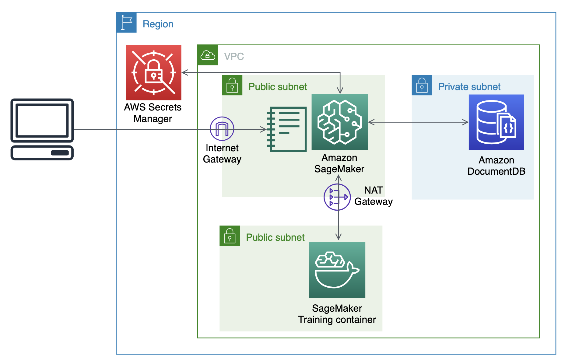
Prepare protein structures and properties and ingest the data into Amazon DocumentDB
All the subsequent code in this section is in the Jupyter notebook Prepare_data.ipynb in the SageMaker instance created in your CloudFormation stack.
This notebook handles the procedures required for preparing and ingesting protein structure data into Amazon DocumentDB.
We first download predicted protein structures from AlphaFold DB in PDB format and the matching experimental structures from the Protein Data Bank.
For demonstration purposes, we only use proteins from the thermophilic archaean Methanocaldococcus jannaschii, which has the smallest proteome of 1,773 proteins for us to work with. You are welcome to try using proteins from other species.
We connect to an Amazon DocumentDB cluster by retrieving the credentials stored in Secrets Manager:
After we set up the connection to Amazon DocumentDB, we parse the PDB files into JSON records to ingest into the database.
We provide utility functions required for parsing PDB files in pdb_parse.py. The parse_pdb_file_to_json_record function does the heavy lifting of extracting atomic coordinates from one or multiple peptide chains in a PDB file and returns one or a list of JSON documents, which can be directly ingested into the Amazon DocumentDB collection as a document. See the following code:
After we ingest the parsed protein data into Amazon DocumentDB, we can update the contents of the protein documents. For instance, it makes our model training logistics easier if we add a field indicating whether a protein structure should be used in the training, validation, or test sets.
We first retrieve the all the documents with the field is_AF to stratify documents using an aggregation pipeline:
Next, we use the update_many function to store the split information back to Amazon DocumentDB:
Train a GNN on the protein structures using SageMaker
All the subsequent code in this section is in the Train_and_eval.ipynb notebook in the SageMaker instance created in your CloudFormation stack.
This notebook trains a GNN model on the protein structure datasets stored in the Amazon DocumentDB.
We first need to implement a PyTorch dataset class for our protein dataset capable of retrieving mini-batches of protein documents from Amazon DocumentDB. It’s more efficient to retrieve batches documents by the built-in primary id (_id).
We use the iterable-style dataset by extending the IterableDataset, which pre-fetches the _id and labels of the documents at initialization:
The ProteinDataset performs a database read operation in the __iter__ method. It tries to evenly split the workload if there are multiple workers:
The preceding __iter__ method also converts the atomic coordinates of proteins into DGLGraph objects after they’re loaded from Amazon DocumentDB via the convert_to_graph function. This function constructs a k-nearest neighbor (kNN) graph for the amino acid residues using the 3D coordinates of the C-alpha atoms and adds one-hot encoded node features to represent residue identities:
With the ProteinDataset implemented, we can initialize instances for train, validation, and test datasets and wrap the training instance with BufferedShuffleDataset to enable shuffling.
We further wrap them with torch.utils.data.DataLoader to work with other components of the SageMaker PyTorch Estimator training script.
Next, we implement a simple two-layered graph convolution network (GCN) with a global attention pooling layer for ease of interpretation:
Afterwards, we can train this GCN on the ProteinDataset instance for a binary classification task of predicting whether a protein structure is predicted by AlphaFold or not. We use binary cross entropy as the objective function and Adam optimizer for stochastic gradient optimization. The full training script can be found in src/main.py.
Next, we set up the SageMaker PyTorch Estimator to handle the training job. To allow the managed Docker container initiated by SageMaker to connect to Amazon DocumentDB, we need to configure the subnet and security group for the Estimator.
We retrieve the subnet ID where the Network Address Translation (NAT) gateway resides, as well as the security group ID of our Amazon DocumentDB cluster by name:
Load and evaluate the trained GNN model
When the training job is complete, we can load the trained GCN model and perform some in-depth evaluation.
The codes for the following steps are also available in the notebook Train_and_eval.ipynb.
SageMaker training jobs save the model artifacts into the default S3 bucket, the URI of which can be accessed from the estimator.model_data attribute. We can also navigate to the Training jobs page on the SageMaker console to find the trained model to evaluate.
For research purposes, we can load the model artifact (learned parameters) into a PyTorch state_dict using the following function:
Next, we perform quantitative model evaluation on the full test set by calculating accuracy:
We found our GCN model achieved an accuracy of 74.3%, whereas the dummy baseline model making predictions based on class priors only achieved 56.3%.
We’re also interested in interpretability of our GCN model. Because we implement a global attention pooling layer, we can compute the attention scores across nodes to explain specific predictions made by the model.
Next, we compute the attention scores and overlay them on the protein graphs for a pair of structures (AlphaFold predicted and experimental) from the same peptide:
The preceding codes produce the following protein graphs overlaid with attention scores on the nodes. We find the model’s global attentive pooling layer can highlight certain residues in the protein graph as being important for making the prediction of whether the protein structure is predicted by AlphaFold. This indicates that these residues may have distinctive graph topologies in predicted and experimental protein structures.
In summary, we showcase a scalable deep learning solution to train GNNs on protein structures stored in Amazon DocumentDB. Although the tutorial only uses thousands of proteins for training, this solution is scalable to millions of proteins. Unlike other approaches such as serializing the entire protein dataset, our approach transfers the memory-heavy workloads to the database, making the memory complexity for the training jobs O(batch_size), which is independent of the total number of proteins to train.
Clean up
To avoid incurring future charges, delete the CloudFormation stack you created. This removes all the resources you provisioned using the CloudFormation template, including the VPC, Amazon DocumentDB cluster, and SageMaker instance. For instructions, see Deleting a stack on the AWS CloudFormation console.
Conclusion
We described a cloud-based deep learning architecture scalable to millions of protein structures by storing them in Amazon DocumentDB and efficiently retrieving mini-batches of data from SageMaker.
To learn more about the use of GNN in protein property predictions, check out our recent publication LM-GVP, A Generalizable Deep Learning Framework for Protein Property Prediction from Sequence and Structure.
About the Authors
Zichen Wang, PhD, is an Applied Scientist in the Amazon Machine Learning Solutions Lab. With several years of research experience in developing ML and statistical methods using biological and medical data, he works with customers across various verticals to solve their ML problems.
Selvan Senthivel is a Senior ML Engineer with the Amazon ML Solutions Lab at AWS, focusing on helping customers on machine learning, deep learning problems, and end-to-end ML solutions. He was a founding engineering lead of Amazon Comprehend Medical and contributed to the design and architecture of multiple AWS AI services.
Read MoreAWS Machine Learning Blog