

The last few years have seen rapid development in the field of natural language processing (NLP). While hardware has improved, such as with the latest generation of accelerators from NVIDIA and Amazon, advanced machine learning (ML) practitioners still regularly run into issues scaling their large language models across multiple GPU’s.
In this blog post, we briefly summarize the rise of large- and small- scale NLP models, primarily through the abstraction provided by Hugging Face and with the modular backend of Amazon SageMaker. In particular we highlight the launch of four additional features within the SageMaker model parallel library that unlock 175 billion parameter NLP model pretraining and fine-tuning for customers.
We used this library on the SageMaker training platform and achieved a throughput of 32 samples per second on 120 ml.p4d.24xlarge instances and 175 billion parameters. We anticipate that if we increased this up to 240 instances, the full model would take 25 days to train.
For more information about model parallelism, see the paper Amazon SageMaker Model Parallelism: A General and Flexible Framework for Large Model Training.
You can also see the GPT2 notebook we used to generate these performance numbers on our GitHub repository.
To learn more about how to use the new features within SageMaker model parallel, refer to Extended Features of the SageMaker Model Parallel Library for PyTorch, and Use with the SageMaker Python SDK.
NLP on Amazon SageMaker – Hugging Face and model parallelism
If you’re new to Hugging Face and NLP, the biggest highlight you need to know is that applications using natural language processing (NLP) are starting to achieve human level performance. This is largely driven by a learning mechanism, called attention, which gave rise to a deep learning model, called the transformer, that is much more scalable than previous deep learning sequential methods. The now-famous BERT model was developed to capitalize on the transformer, and developed several useful NLP tactics along the way. Transformers and the suite of models, both within and outside of NLP, which have all been inspired by BERT, are the primary engine behind your Google search results, in your Google translate results, and a host of new startups.
SageMaker and Hugging Face partnered to make this easier for customers than ever before. We’ve launched Hugging Face deep learning containers (DLC’s) for you to train and host pre-trained models directly from Hugging Face’s repository of over 26,000 models. We’ve launched the SageMaker Training Compiler for you to speed up the runtime of your Hugging Face training loops by up to 50%. We’ve also integrated the Hugging Face flagship Transformers SDK with our distributed training libraries to make scaling out your NLP models easier than ever before.
For more information about Hugging Face Transformer models on Amazon SageMaker, see Support for Hugging Face Transformer Models.
New features for large-scale NLP model training with the SageMaker model parallel library
At AWS re:Invent 2020, SageMaker launched distributed libraries that provide the best performance on the cloud for training computer vision models like Mask-RCNN and NLP models like T5-3B. This is possible through enhanced communication primitives that are 20-40% faster than NCCL on AWS, and model distribution techniques that enable extremely large language models to scale across tens to hundreds to thousands of GPUs.
The SageMaker model parallel library (SMP) has always given you the ability to take your predefined NLP model in PyTorch, be that through Hugging Face or elsewhere, and partition that model onto multiple GPUs in your cluster. Said another way, SMP breaks up your model into smaller chunks so you don’t experience out of memory (OOM) errors. We’re pleased to add additional memory-saving techniques that are critical for large scale models, namely:
Tensor parallelism
Optimizer state sharding
Activation checkpointing
Activation offloading
You can combine these four features can be combined to utilize memory more efficiently and train the next generation of extreme scale NLP models.
Distributed training and tensor parallelism
To understand tensor parallelism, it’s helpful to know that there are many kinds of distributed training, or parallelism. You’re probably already familiar with the most common type, data parallelism. The core of data parallelism works like this: you add an extra node to your cluster, such as going from one to two ml.EC2 instances in your SageMaker estimator. Then, you use a data parallel framework like Horovod, PyTorch Distributed Data Parallel, or SageMaker Distributed. This creates replicas of your model, one per accelerator, and handles sharding out the data to each node, along with bringing all the results together during the back propagation step of your neural network. Think distributed gradient descent. Data parallelism is also popular within servers; you’re sharding data into all the GPUs, and occasionally CPUs, on all of your nodes. The following diagram illustrates data parallelism.
Model parallelism is slightly different. Instead of making copies of the same model, we split your model into pieces. Then we manage the running it, so your data is still flowing through your neural network in exactly the same way mathematically, but different pieces of your model are sitting on different GPUs. If you’re using an ml.p3.8xlarge, you’ve got four NVIDIA V100’s, so you’d probably want to shard your model into 4 pieces, one piece per GPU. If you jump up to two ml.p4d.24xlarge’s, that’s 16 A100’s total in your cluster, so you might break your model into 16 pieces. This is also sometimes called pipeline parallelism. That’s because the set of layers in the network are partitioned across GPUs, and run in a pipelined manner to maximize the GPU utilization. The following diagram illustrates model parallelism.
To make model parallelism happen at scale, we need a third type of distribution: tensor parallelism. Tensor parallelism applies the same concepts at one step further—we break apart the largest layers of your neural network and place parts of the layers themselves on different devices. This is relevant when you’re working with 175 billion parameters or more, and trying to fit even a few records into RAM, along with parts of your model, to train that transformer. The following diagram illustrates tensor parallelism.
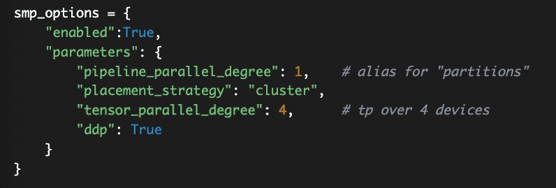
To enable tensor parallelism, set it within the smp options you pass to your estimator.
In the preceding code, pipeline_parallel_degree describes into how many segments your model should be sharded, based on the pipeline parallelism we discussed above. Another word for this is partitions.
To enable tensor parallelism, set tensor_parallel_degree to your desired level. Make sure you’re picking a number equal to or smaller than the number of GPU’s per instance, so no greater than 8 for the ml.p4d.24xlarge machines. For additional script changes, refer to Run a SageMaker Distributed Model Parallel Training Job with Tensor Parallelism.
The ddp parameter refers to distributed data parallel. You typically enable this if you’re using data parallelism or tensor parallelism, because the model parallelism library relies on DDP for these features.
Optimizer state sharding, activation offloading and checkpoints
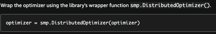
If you have an extremely large model, you also need an extremely large optimizer state. Prepping your optimizer for SMP is straightforward: simply pick it up from disk in your script and load it into the smp.DistributedOptimizer() object.
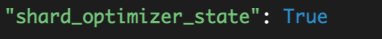
Make sure you enable this at the estimator by setting shard_optimizer_state to True in the smp_options you use to configure SMP:
Similar to tensor and pipeline parallelism, SMP profiles your model and your world size (the total number of GPUs in all of your training nodes), to find the best placement strategies.
In deep learning the intermediate layer outputs are also called activations, and these need to be stored during forward pass. This is because they need to be used for gradient computation in the backward pass. In a large model, storing all these activations simultaneously in memory can create significant memory bottlenecks. To address this bottleneck, you can use activation checkpointing, the third new feature in the SageMaker model parallelism library. Activation checkpointing, or gradient checkpointing, is a technique to reduce memory usage by clearing activations of certain layers and recomputing them during a backward pass. This effectively trades extra computation time for reduced memory usage.
Lastly, activation offloading directly uses activation checkpointing. It’s a strategy to keep only a few tensor activations on the GPU RAM during the model training. Specifically, we move the checkpointed activations to CPU memory during the forward pass and load them back to GPU for the backward pass of a specific micro-batch.
Micro-batches and placement strategies
Other topics that sometimes cause customers confusion are micro-batches and placement strategies. Both of these are hyperparameters you can supply to the SageMaker model parallel library. Specifically micro-batches are relevant when implementing models that rely on pipeline parallelism, such as those at least 30 billion parameters in size or more.
Micro-batches are subsets of minibatches. When your model is in its training loop, you define a certain number of records to pick up and pass forward and backward through the layers–this is called a minibatch, or sometimes just a batch. A full pass through your dataset is called an epoch. To run forward and backward passes with pipeline parallelism, SageMaker model parallel library shards the batches into smaller subsets called micro-batches, which are run one at a time to maximize GPU utilization. The resultant, much smaller set of examples per-GPU, is called a micro-batch. In our GPT-2 example, we added a default of 1 microbatch directly to the training script.
As you scale up your training configuration, you are strongly recommended to change your batch size and micro-batch size accordingly. This is the only way to ensure good performance: you must consider batch size and micro-batch sizes as a function of your overall world size when relying on pipeline parallelism.
Placement strategies are how to tell SageMaker physically where to place your model partitions. If you’re using both model parallel and data parallel, setting placement_strategy to “cluster” places model replicas in device ID’s (GPUs) that are physically close to each other. However, if you really want to be more prescriptive about your parallelism strategy, you can break it down into a single string with different combinations of three letters: D for data parallelism, P indicates pipeline parallelism, and T for tensor parallelism. We generally recommend keeping the default placement of “cluster”, because this is most appropriate for large scale model training. The “cluster” placement corresponds to “DPT“.
For more information about placement strategies, see Placement Strategy with Tensor Parallelism.
Example use case
Let’s imagine you have one ml.p3.16xlarge in your training job. That gives you 8 NVIDIA V100’s per node. Remember, every time you add an extra instance, you experience additional bandwidth overhead, so it’s always better to have more GP’Us on a single node. In this case, you’re better off with one ml.p3.16xlarge than, for example, two ml.p3.8xlarges. Even though the number of GPUs is the same, the extra bandwidth overhead of the extra node slows down your throughput.
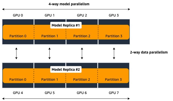
The following diagram illustrates four-way model parallelism, combined with two-way data parallelism. This means you actually have two replicas of your model (think data parallel), with each of them partitioned across four GPU’s (model parallel).
If any of those model partitions are too large to fit onto a single GPU, you can add an extra type of distribution–tensor parallelism–to spit it and utilize both devices.
Conclusion
In this blog post we discussed SageMaker distributed training libraries, especially focusing on model parallelism. We shared performance benchmarks from our latest test, achieving 32 samples per second across 120 ml.p4d.24xlarge instances and 175B parameters on Amazon SageMaker. We anticipate that if we increased this to 240 p4 instances we could train a 175B parameter model in 25 days.
We also discussed the newest features the enable large-scale training, namely tensor parallelism, optimizer state sharding, activation checkpointing, and activation offloading. We shared some tips and tricks for enabling this through training on Amazon SageMaker.
Try it out yourself using the same notebook that generated our numbers, which is available on GitHub here. You can also request more GPUs for your AWS account through requesting a service limit approval right here.
About the Authors
Emily Webber joined AWS just after SageMaker launched, and has been trying to tell the world about it ever since! Outside of building new ML experiences for customers, Emily enjoys meditating and studying Tibetan Buddhism.
Aditya Bindal is a Senior Product Manager for AWS Deep Learning. He works on products that make it easier for customers to train deep learning models on AWS. In his spare time, he enjoys spending time with his daughter, playing tennis, reading historical fiction, and traveling.
Luis Quintela is the Software Developer Manager for the AWS SageMaker model parallel library. In his spare time, he can be found riding his Harley in the SF Bay Area.
Read MoreAWS Machine Learning Blog