Method of Lagrange Multipliers: The Theory Behind Support Vector Machines (Part 2: The Non-Separable Case)

Last Updated on December 3, 2021

This tutorial is an extension of Method Of Lagrange Multipliers: The Theory Behind Support Vector Machines (Part 1: The Separable Case)) and explains the non-separable case. In real life problems positive and negative training examples may not be completely separable by a linear decision boundary. This tutorial explains how a soft margin can be built that tolerates a certain amount of errors.

In this tutorial, we’ll cover the basics of a linear SVM. We won’t go into details of non-linear SVMs derived using the kernel trick. The content is enough to understand the basic mathematical model behind an SVM classifier.

After completing this tutorial, you will know:

Concept of a soft margin
How to maximize the margin while allowing mistakes in classification
How to formulate the optimization problem and compute the Lagrange dual

Let’s get started.

Tutorial Overview

This tutorial is divided into 2 parts; they are:

The solution of the SVM problem for the case where positive and negative examples are not linearly separable
The separating hyperplane and the corresponding relaxed constraints
The quadratic optimization problem for finding the soft margin

A worked example

Pre-requisites

For this tutorial, it is assumed that you are already familiar with the following topics. You can click on the individual links to get more information.

A Gentle Introduction to Optimization / Mathematical Programming
A Gentle Introduction To Method Of Lagrange Multipliers
Lagrange Multiplier Approach with Inequality Constraints
Method Of Lagrange Multipliers: The Theory Behind Support Vector Machines (Part 1: The Separable Case))

Notations Used In This Tutorial

This is a continuation of Part 1, so the same notations will be used.

$m$: Total training points
$x$: Data point, which is an $n$-dimensional vector. Each dimension is indexed by j.
$x^+$: Positive example
$x^-$: Negative example
$i$: Subscript used to index the training points. $0 leq i < m$
$j$: Subscript to index a dimension of the data point. $1 leq j leq n$
$t$: Label of data points. It is an m-dimensional vector
$T$: Transpose operator
$w$: Weight vector denoting the coefficients of the hyperplane. It is an $n$-dimensional vector
$alpha$: Vector of Lagrange multipliers, an $m$-dimensional vector
$mu$: Vector of Lagrange multipliers, again an $m$-dimensional vector
$xi$: Error in classification. An $m$-dimensional vector

The Separating Hyperplane and Relaxing the Constraints

Let’s find a separating hyperplane between the positive and negative examples. Just to recall, the separating hyperplane is given by the following expression, with (w_j) being the coefficients and (w_0) being the arbitrary constant that determines the distance of the hyperplane from the origin:

$$
w^T x_i + w_0 = 0
$$

As we allow positive and negative examples to lie on the wrong side of the hyperplane, we have a set of relaxed constraints. Defining $xi_i geq 0, forall i$, for positive examples we require:

$$
w^T x_i^+ + w_0 geq 1 – xi_i
$$

Also for negative examples we require:

$$
w^T x_i^- + w_0 leq -1 + xi_i
$$

Combining the above two constraints by using the class label $t_i in {-1,+1}$ we have the following constraint for all points:

$$
t_i(w^T x_i + w_0) geq 1 – xi_i
$$

The variable $xi$ allows more flexibility in our model. It has the following interpretations:

$xi_i =0$: This means that $x_i$ is correctly classified and this data point is on the correct side of the hyperplane and away from the margin.
$0 < xi_i < 1$: When this condition is met, $x_i$ lies on the correct side of the hyperplane but inside the margin.
$xi_i > 0$: Satisfying this condition implies that $x_i$ is misclassified.

Hence, $xi$ quantifies the errors in the classification of training points. We can define the soft error as:

$$
E_{soft} = sum_i xi_i
$$

The Quadratic Programming Problem

We are now in a position to formulate the objective function along with the constraints on it. We still want to maximize the margin, i.e., we want to minimize the norm of the weight vector. Along with this, we also want to keep the soft error as small as possible. Hence, now our new objective function is given by the following expression, with $C$ being a user defined constant and represents the penalty factor or the regularization constant.

$$
frac{1}{2}||w||^2 + C sum_i xi_i
$$

The overall quadratic programming problem is, therefore, given by the following expression:

$$
min_w frac{1}{2}||w||^2 + C sum_i xi_i ;text{ subject to } t_i(w^Tx_i+w_0) geq +1 – xi_i, forall i ; text{ and } xi_i geq 0, forall i
$$

The Role of C, the Regularization Constant

To understand the penalty factor $C$, consider the product term $C sum_i xi_i$, which has to be minimized. If C is kept large, then the soft margin $sum_i xi_i$ would automatically be small. If $C$ is close to zero, then we are allowing the soft margin to be large making the overall product small.

In short, a large value of $C$ means we have a high penalty on errors and hence our model is not allowed to make too many mistakes in classification. A small value of $C$ allows the errors to grow.

Solution Via The Method Of Lagrange Multipliers

Let’s use the method of Lagrange multipliers to solve the quadratic programming problem that we formulated earlier. The Lagrange function is given by:

$$
L(w, w_0, alpha, mu) = frac{1}{2}||w||^2 + sum_i alpha_ibig(t_i(w^Tx_i+w_0) – 1 + xi_ibig) – sum_i mu_i xi_i
$$

To solve the above, we set the following:
begin{equation}
frac{partial L}{ partial w} = 0, \
frac{partial L}{ partial alpha} = 0, \
frac{partial L}{ partial w_0} = 0, \
frac{partial L}{ partial mu} = 0 \
end{equation}

Solving the above gives us:
$$
w = sum_i alpha_i t_i x_i
$$
and
$$
0= C – alpha_i – mu_i
$$

Substitute the above in the Lagrange function gives us the following optimization problem, also called the dual:

$$
L_d = -frac{1}{2} sum_i sum_k alpha_i alpha_k t_i t_k (x_i)^T (x_k) + sum_i alpha_i
$$

We have to maximize the above subject to the following constraints:

begin{equation}
sum_i alpha_i t_i = 0 \ text{ and }
0 leq alpha_i leq C, forall i
end{equation}

Similar to the separable case, we have an expression for $w$ in terms of Lagrange multipliers. The objective function involves no $w$ term. There is a Lagrange multiplier $alpha$ and $mu$ associated with each data point.

Interpretation of the Mathematical Model and Computation of $w_0$

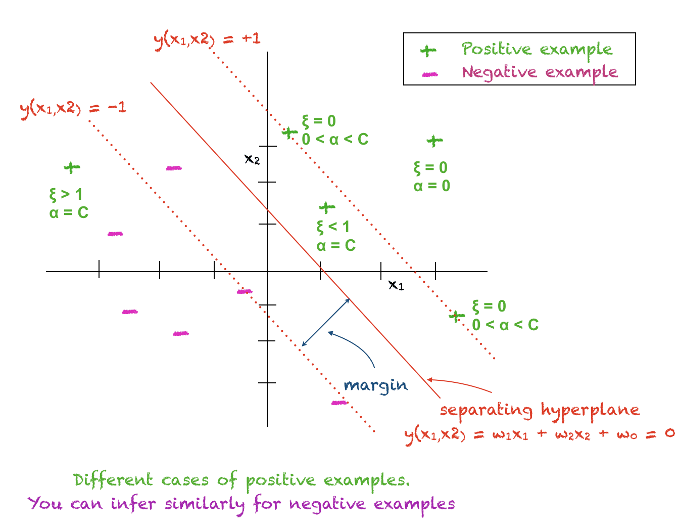
Following cases are true for each training data point $x_i$:

$alpha_i = 0$: The ith training point lies on the correct side of the hyperplane away from the margin. This point plays no role in the classification of a test point.
$0 < alpha_i < C$: The ith training point is a support vector and lies on the margin. For this point $xi_i = 0$ and $t_i(w^T x_i + w_0) = 1$ and hence it can be used to compute $w_0$. In practice $w_0$ is computed from all support vectors and an average is taken.
$alpha_i = C$: The ith training point is either inside the margin on the correct side of the hyperplane or this point is on the wrong side of the hyperplane.

The picture below will help you understand the above concepts:

Deciding The Classification of a Test Point

The classification of any test point $x$ can be determined using this expression:

$$
y(x) = sum_i alpha_i t_i x^T x_i + w_0
$$

A positive value of $y(x)$ implies $xin+1$ and a negative value means $xin-1$. Hence, the predicted class of a test point is the sign of $y(x)$.

Karush-Kuhn-Tucker Conditions

Karush-Kuhn-Tucker (KKT) conditions are satisfied by the above constrained optimization problem as given by:
begin{eqnarray}
alpha_i &geq& 0 \
t_i y(x_i) -1 + xi_i &geq& 0 \
alpha_i(t_i y(x_i) -1 + xi_i) &=& 0 \
mu_i geq 0 \
xi_i geq 0 \
mu_ixi_i = 0
end{eqnarray}

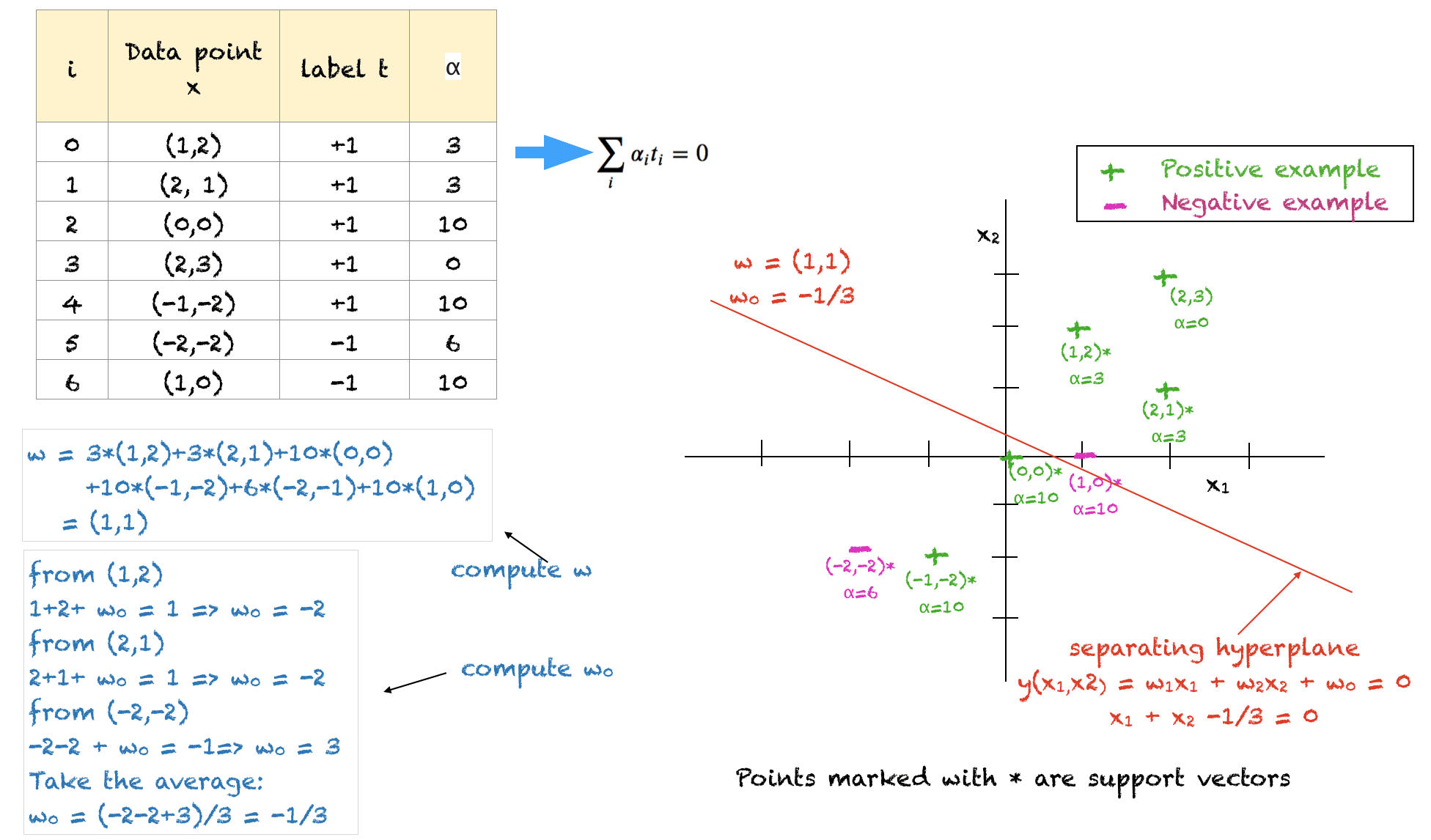
A Solved Example

Shown above is a solved example for 2D training points to illustrate all the concepts. A few things to note about this solution are:

The training data points and their corresponding labels act as input
The user defined constant $C$ is set to 10
The solution satisfies all the constraints, however, it is not the optimal solution
We have to make sure that all the $alpha$ lie between 0 and C
The sum of alphas of all negative examples should equal the sum of alphas of all positive examples
The points (1,2), (2,1) and (-2,-2) lie on the soft margin on the correct side of the hyperplane. Their values have been arbitrarily set to 3, 3 and 6 respectively to balance the problem and satisfy the constraints.
The points with $alpha=C=10$ lie either inside the margin or on the wrong side of the hyperplane

Further Reading

This section provides more resources on the topic if you are looking to go deeper.

Books

Pattern Recognition and Machine Learning by Christopher M. Bishop

Articles

Support Vector Machines for Machine Learning
A Tutorial on Support Vector Machines for Pattern Recognition by Christopher J.C. Burges

Summary

In this tutorial, you discovered the method of Lagrange multipliers for finding the soft margin in an SVM classifier.

Specifically, you learned:

How to formulate the optimization problem for the non-separable case
How to find the hyperplane and the soft margin using the method of Lagrange multipliers
How to find the equation of the separating hyperplane for very simple problems

Do you have any questions about SVMs discussed in this post? Ask your questions in the comments below and I will do my best to answer.

The post Method of Lagrange Multipliers: The Theory Behind Support Vector Machines (Part 2: The Non-Separable Case) appeared first on Machine Learning Mastery.

Read MoreMachine Learning Mastery