

Model training forms the core of any machine learning (ML) project, and having a trained ML model is essential to adding intelligence to a modern application. A performant model is the output of a rigorous and diligent data science methodology. Not implementing a proper model training process can lead to high infrastructure and personnel costs because it underlines the experimental phase of the ML process and by nature tends to be highly iterative.
Generally speaking, training a model from scratch is time-consuming and compute intensive. When the training data is small, we can’t expect to train a very performant model. A better alternative is to fine-tune a pretrained model on the target dataset. For certain use cases, Amazon SageMaker provides high-quality pretrained models that were trained on very large datasets. Fine-tuning these models takes a fraction of the training time compared to training a model from scratch.
To validate this assertion, we ran a study using built-in algorithms with pretrained models. We also compared two types of pretrained models within Amazon SageMaker Studio, Type 1 (legacy) and Type 2 (latest), against a model trained from scratch using Defect Detection Network (DDN) with regards to training time and infrastructure cost. To demonstrate the training process, we used the default detection dataset from the post Visual inspection automation using Amazon SageMaker JumpStart. This post showcases the results of the study. We also provide a Studio notebook, which you can modify to run the experiments using your own dataset and an algorithm or model of your choosing.
Model training in Studio
SageMaker is a fully managed ML service. With SageMaker, data scientists and developers can quickly and easily build and train ML models, and then directly deploy them into a production-ready hosted environment.
There are many ways with which you can train ML models using SageMaker, such as using Amazon SageMaker Debugger, Spark MLLib, or using custom Python code with TensorFlow, PyTorch, or Apache MXNet. You can also bring your own custom algorithm or choose an algorithm from AWS Marketplace.
Furthermore, SageMaker provides a suite of built-in algorithms, pre-trained models, and pre-built solution templates to help data scientists and ML practitioners get started on training and deploying ML models quickly.
You can use built-in algorithms for either classification or regression problems, or for a variety of unsupervised learning tasks. Other built-in algorithms include text analysis and image processing. You can train a model from scratch using a built-in algorithm for a specific use case. For a full list of available built-in algorithms, see Common Information About Built-in Algorithms.
Some built-in algorithms also include pre-trained models for popular problem types that use the SageMaker SDK as well as Studio. These pre-trained models can greatly reduce the training time as well as infrastructure cost for common use cases such as semantic segmentation, object detection, text summarization, and question answering. For a complete list of pre-trained models, see Models.
For choosing the best model, SageMaker automatic model tuning, also known as hyperparameter tuning or hyperparameter optimization (HPO), can be very useful because it finds the best version of a model by running a slew of training jobs on your dataset using the algorithm and hyperparameters that you specify. Depending on the number of hyperparameters and the size of the search space, finding the best model can require thousands or even tens of thousands of training runs. Automatic model tuning provides a built-in HPO algorithm that removes the undifferentiated heavy lifting required to build your own HPO algorithm. Automatic model tuning provides the option of parallelizing model runs in order to reduce the time and cost of finding the best fit.
After the automatic model tuning has completed multiple runs for a set of hyperparameters, it chooses the hyperparameter values that result in the model with the best performance, as measured by the loss function specific to the model.
Training and validation loss is just one of the metrics needed to pick the best model for the use case. With so many options, it’s not always easy to make the right choice, and picking the best model boils down to the training time, cost of infrastructure, complexity, and quality of the resulting model, among other factors. There are other extraneous costs such as platform and personnel costs that we don’t take into account for this study.
In the subsequent sections, we discuss the study design and the results.
Dataset
We use the NEU-CLS dataset and a detector on the NEU-DET dataset. This dataset contains 1,800 images and 4,189 bounding boxes in total. The type of defects in our dataset are as follows:
Crazing (class: Cr, label: 0)
Inclusion (class: In, label: 1)
Pitted surface (class: PS, label: 2)
Patches (class: Pa, label: 3)
Rolled-in scale (class: RS, label: 4)
Scratches (class: Sc, label: 5)
For more details about the dataset, refer to Visual inspection automation using Amazon SageMaker JumpStart.
Models
We introduced the Defect Detection Network in the post Visual inspection automation using Amazon SageMaker JumpStart. We trained this model from scratch with the default hyperparameters, so we could have a benchmark to evaluate the rest of the models.
For object detection use cases, SageMaker provides the following set of built-in object models:
Type 1 (legacy) – Uses a built-in legacy object detection algorithm and uses the Single Shot multibox Detector (SSD) model with either a VGG or ResNet backbone, and was pre-trained on the ImageNet dataset.
Type 2 (latest) – Provides nine pre-trained object detection models, including eight SSD models and one FasterRCNN model. These models use VGG, ResNet, or MobileNet as the backbone, and were pre-trained on COCO, VOC, or FPN datasets.
Aside from training a model from scratch, we used these models to evaluate four approaches that typically reflect an ML model training process. The output of each approach is a trained ML model. In cases 1 and 3, a set of fixed hyperparameters are provided to train a single model, whereas in cases 2 and 4, SageMaker produces the best model and the set of hyperparameters that led to the best fit.
Type 1 (legacy) model – We use the model with a ResNet backbone, which is pre-trained on ImageNet with default hyperparameters and no optimizer.
Fine-tune Type 1 (legacy) with HPO – Now we run HPO to find better hyperparameters that lead to a better model. For a list of all parameters you can fine-tune, refer to Tune an Object Detection Model. In this notebook, we only fine-tune learning rate, momentum, and weight decay. We use automatic model tuning to run HPO. We need to provide hyperparameter ranges for learning rate, momentum, and weight decay. Automatic model tuning will monitor the log and parse the objective metrics. For object detection, we use Mean Average Precision (mAP) on the validation dataset as our metric.
Fine-tune Type 2 (latest) model – For the Type 2 (latest) object detection model, we follow the instructions in Fine-tune a Model and Deploy to a SageMaker Endpoint and use standard SageMaker APIs. You can find all fine-tunable Type 2 (latest) object detection models in the Built-in Algorithms with pre-trained Model table and set FineTunable?=True. Currently, there are nine fine-tunable object detection models. We use the one with the VGG backend and pretrained on VOC dataset. We fine-tune using a set of static hyperparameters.
Fine-tune Type 2 (latest) model with HPO – We provide a range for the ADAM learning rate; the rest of the hyperparameters stay default. Also, note that the Type 2 (latest) model training reports Val_CrossEntropy loss and Val_SmoothL1 loss instead of mAP on the validation dataset. Because we can only specify one evaluation metric for automatic model tuning, we choose to minimize Val_CrossEntropy.
For details on the hyperparameters, you can go through the Studio notebook.
Metrics
Next, we compare the results from the approaches based on important metrics and the infrastructure cost:
Loss function difference across models – All the different algorithms define the same loss function for object detection task: cross-entropy and smooth L1 loss. However, we use them differently:
The Type 1 (legacy) object detection algorithm has defined mAP on the validation data, and we use it as the metric to find a training job that maximizes mAP.
The Type 2 (latest) object detection algorithm, however, doesn’t define mAP. Instead, it defines Val_SmoothL1 loss and Val_CrossEntropy loss on the validation data. During model training with HPO, we need to specify one metric for automatic model tuning to monitor and parse. Therefore, we use Val_CrossEntropy loss as the metric and find the training job that minimizes it.
Validation metric (mAP) – We use the mAP on the validation dataset as our metric, where average precision is the average of precision and recall. mAP is the standard evaluation metric used in the COCO challenge for object detection tasks. For more information about the applicability of mAP for object detection, refer to mAP (mean Average Precision) for Object Detection. Because there is a difference in loss function between Type 1 and Type 2 models, we manually calculate the mAP for each type of model on the test dataset. We accomplish this by deploying the models behind a SageMaker endpoint and calling the model endpoint to score on the subset of the dataset. The results are then compared against the ground truth to calculate the mAP for each model type.
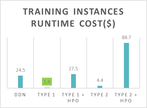
Training Instances Runtime cost – For simplicity, we only report the infrastructure cost incurred for each of the four approaches highlighted in the previous section. The cost is reported in dollars and calculated based on the runtime of the underlying Amazon Elastic Compute Cloud (Amazon EC2) instances.
Notebook
The Studio notebook is available on GitHub.
Results
The steel surface dataset has a total of 1,800 images in six categories. As discussed in the previous section, because there is a difference in the loss function that Type 1 (legacy) and Type 2 (latest) models maximize to find the best model, we first perform a train/test split on the dataset. In the final phase of the study, we run inference on the test dataset, so that we can compare across the four approaches using the same metric (mAP).
The test set contains 20% of the original dataset, which we randomly allocate from the full dataset. The remaining 80% is used for the model training phase, which requires us to define the training as well as the validation dataset. Therefore, for the training phase, we do a further 80/20 split on the data, where 80% of the training data is used for training and 20% for validation. See the following table.
Data
Number of Samples
Percentage of Original Dataset
Full
1,800
100
Train
1,152
64
Validation
288
16
Test
360
20
The output of each of the four approaches was a trained ML model. We plot the results from each of the four approaches alongside the bounding boxes from ground truth as well as the DDN model. The following plot also shows the confidence score for the class prediction.
A confidence score is provided as an evaluation standard. This confidence score shows the probability of the object of interest being detected correctly by the algorithm and is given as a percentage. The scores are taken on the mAP at different IoU (Intersection over Union) thresholds.
For the purpose of generating the mAP score against the test dataset, we deployed each model behind its own SageMaker real-time endpoint. Each inferencing test produced a mAP score.
A larger mAP score implies a higher accuracy of the model test results. Clearly, the Type 2 (latest) models outperforms the Type 1 (legacy) models in regards to accuracy, with or without using HPO. Type 2 with HPO has a slighter edge (mAP 0.375) over one without HPO (mAP 0.371).
We also measured the cost of training for each of the four approaches. We used the P3 instance types, specifically the ml.p3.2xlarge instances for each of the approaches. Each ml.p3.2xlarge instance costs $3.06/hour. Both the inference test mAP score and the cost of training are summarized in the following chart for comparison.
For simplicity, we did a cost comparison on the runtime of the training instances only.
For a more granular estimate of the total cost incurred, including the cost of Studio notebooks as well as the real-time endpoints used for inferencing, refer to the AWS Pricing Calculator for SageMaker.
The results indicate considerable gains in accuracy when moving from the Type 1 (legacy) to Type 2 (latest) model. The mAP score went up from 0.067 to 0.371 without using HPO and 0.226 to 0.375 with HPO respectively. The Type 2 model also took longer to train with the same instance type, implying that the accuracy gains also meant higher infrastructure cost. However, all mentioned approaches outperformed the DDN model (introduced in Visual inspection automation using Amazon SageMaker JumpStart) on all metrics. Training the Type 1 (legacy) model took 34 minutes, the Type 2 (latest) model took 1 hour, and the DDN model took over 8 hours. This indicates that fine-tuning a pre-trained model is much more efficient than training a model from scratch.
We also found that HPO (SageMaker automatic model tuning) is extremely effective, especially for models with large hyperparameter search spaces with 4x improvement in mAP score for Type 1 (legacy) model. We noted that we yielded much better model accuracy results when fine-tuning on three hyperparameters (learning rate, momentum, and weight decay) for the Type 1 (legacy) models as opposed to only one hyperparameter (ADAM learning rate) for the Type 2 (latest) model. This is because there is a relatively larger search space and therefore more room for improvement for the Type 1 (legacy) model. However, we need to trade off model performance with infrastructure cost and training time when running HPO.
Conclusion
In this post, we walked through the many ML model training options available with SageMaker and focused specifically on SageMaker built-in algorithms and pre-trained models. We introduced Type 1 (legacy) and Type 2 (latest) models. The built-in Sagemaker object detection models discussed in this post were pre-trained on large-scale datasets—the ImageNet dataset includes 14,197,122 images for 21,841 categories, and the PASCAL VOC dataset includes 11,530 images for 20 categories. The pre-trained models have learned rich and diverse low-level features, and can efficiently transfer knowledge to fine-tuned models and focus on learning high-level semantic features for the target dataset. You can find all built-in algorithms and fine-tunable pre-trained models at Built-in Algorithms with pre-trained Model Table and choose one for your use case. The use cases span from text summarization and question answering to computer vision and regression or classification.
In the beginning, we made an assertion that fine-tuning a SageMaker pre-trained model will take a fraction of training time that training a model from scratch. We trained a DNN model from scratch and introduced two types of SageMaker Built-in algorithms with pretrained models: Type (legacy) and Type 2 (latest). We further showcased four approaches, two of which used SageMaker automated model tuning, and finally arrived at the most performant model. When considering both training time as well as runtime cost, all SageMaker built-in algorithms outperformed the DDN model, thereby validating our assertion.
Although both Type 1 (legacy) and Type 2 (latest) outperformed training the DDN model from scratch, visual and numerical comparison confirmed that the Type 2 (latest) model and Type 2 (latest) model with HPO outperforms Type 1 (legacy) models. HPO had a big impact on accuracy for Type 1 models; however, it saw modest gains using HPO for Type 2 models, due to a constricted hyperparameter space.
In summary, for certain use cases, fine-tuning a pretrained model is both more efficient and more performant. We suggest taking advantage of the pre-trained Sagemaker built-in pretrained models and fine-tune on your target datasets. To get started, you need a Studio environment. For more information, refer to the Studio Development Guide and make sure to enable SageMaker projects and JumpStart. When your Studio setup is complete, navigate to the Studio Launcher to find the full list of JumpStart solutions and models. To recreate or modify the experiment in this post, choose the “Product Defect Detection” solution, which comes prepackaged with the notebook used to experiment, as shown in the following video. After you launch the solution, you can access the mentioned work in the notebook titled visual_object_detection.ipynb.
About the authors
Vedant Jain is a Sr. AI/ML Specialist Solutions Architect, helping customers derive value out of the Machine Learning ecosystem at AWS. Prior to joining AWS, Vedant has held ML/Data Science Specialty positions at various companies such as Databricks, Hortonworks (now Cloudera) & JP Morgan Chase. Outside of his work, Vedant is passionate about making music, using Science to lead a meaningful life & exploring delicious vegetarian cuisine from around the world.
Tao Sun is an Applied Scientist in Amazon Search. He obtained his Ph.D. in Computer Science from University of Massachusetts, Amherst. His research interests lie in deep reinforcement learning and probabilistic modeling. In the past, Tao worked for AWS Sagemaker Reinforcement Learning team and contributed to RL research and applications. Tao is now working on Page Template Optimization at Amazon Search.
Read MoreAWS Machine Learning Blog