

Recommendation systems are one of the most widely adopted machine learning (ML) technologies in real-world applications, ranging from social networks to ecommerce platforms. Users of many online systems rely on recommendation systems to make new friendships, discover new music according to suggested music lists, or even make ecommerce purchase decisions based on the recommended products. In social networks, one common use case is to recommend new friends to a user based on the users’ other connections. Users with common friends likely know each other. Therefore, they should have a higher score for a recommendation system to propose if they haven’t been connected yet.
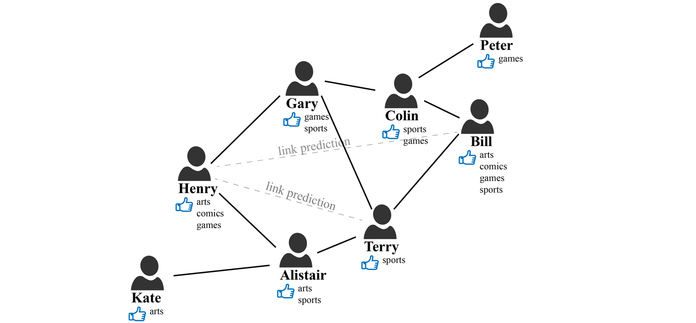
Social networks can naturally be expressed in a graph, where the nodes represent people, and the connections between people, such as friendship or co-workers, are represented by edges. The following illustrates one such social network. Let’s imagine that we have a social network with the members (nodes) Bill, Terry, Henry, Gary, and Alistair. Their relationships are represented by a link (edge), and each person’s interests, such as sports, arts, games, and comics, are represented by node properties.
The objective here is to predict if there is a potential missing link between members. For example, should we recommend a connection between Henry and Terry? Looking at the graph, we can see that they have two mutual friends, Gary and Alistair. Therefore, there is a good chance that Henry and Terry either already knew each other or may get to know each other soon. How about Henry and Bill? They don’t have any mutual friends, but they do have some weak connection through their friends’ connections. In addition, they both have similar interests in arts, comics, and games. Should we promote this connection? All of these questions and intuitions are the core logic of social network recommendation systems.
One possible way to do this is recommending relationships based on graph exploration. In graph query languages, such as Apache TinkerPop Gremlin, the implementation of rule sets such as counting common friends, is relatively easy, and it can be used to determine the link between Henry and Terry. However, these rule sets will be very complicated when we want account for other attributes such as node properties, connection strength, etc. Let’s imagine a rule set to determine the link between Henry and Bill. This rule set must account for their common interests and their weak connections through certain paths in the graph. To increase robustness, we might also need to add a distance factor to favor strong connections and penalize the weak ones. Similarly, we would want a factor to favor common interests. Soon, the rule sets that can reveal complex hidden patterns will become impossible to enumerate.
ML technology lets us discover hidden patterns by learning algorithms. One example is XGBoost, which is widely used for classification or regression tasks. However, algorithms such as XGBoost use a conventional ML approach based on a tabular data format. These approaches aren’t optimized for graph data structures, and they require complex feature engineering to cope with these data patterns.
In the preceding social network example, the graph interaction information is critical to improving the recommendation accuracy. Graph Neural Network (GNN) is a deep learning (DL) framework that can be applied to graph data to perform edge-level, node-level, or graph-level prediction tasks. GNNs can leverage individual node characteristics as well as graph structure information when learning the graph representation and underlying patterns. Therefore, in recent years, GNN-based methods have set new standards on many recommender system benchmarks. See more detailed information in recent research papers: A Comprehensive Survey on Graph Neural Networks and Graph Learning based Recommender Systems: A Review.
The following is one famous example of such a use case. Researchers and engineers at Pinterest have trained Graph Convolutional Neural Networks for Web-Scale Recommender Systems, called PinSage, with three billion nodes representing pins and boards, and 18 billion edges. PinSage generates high-quality embeddings that represent pins (visual bookmarks to online content). These can be used for a wide range of downstream recommendation tasks, such as nearest-neighbor lookups in the learned embedding space for content discovery and recommendations.
In this post, we will walk you through how to use GNNs for recommendation use cases by casting this as a link prediction problem. We’ll also illustrate how Neptune ML can facilitate implementation. We will also provide sample code on GitHub to train your first GNN with Neptune ML, and make recommendation inferences on the demo graph through link prediction tasks.
Link prediction with Graph Neural Networks
Considering the previous social network example, we would like to recommend new friends to Henry. Both Terry and Bill would be good candidates. Terry has more common friends (Gary, Alistair) with Henry but no common interests. While Bill shares common interests (arts, comics, games) with Henry, but no common friends. Which one would be a better recommendation? When framed as a link prediction problem, the task is to assign a score to any possible link between the two nodes. The higher the link score, the more likely this recommendation will converge. By learning link structures already present in the graph, a link prediction model can generalize new link predictions that ‘complete’ the graph.
The parameters of the function f that predicts the link score is learned during the training phase. Since the function f makes a prediction for any two nodes in the graph, the feature vectors associated with the nodes are essential to the learning process. To predict the link score between Henry and Bill, we have a set of raw data features (arts, comics, games) that can represent Henry and Bill. We transform this, along with the connections in the graph, using a GNN network to form new representations known as node embeddings. We can also supplement or replace the initial raw features with vectors from an embedding lookup table that can be learned during the training process. Ideally, the embedded features for Henry and Bill should represent their interests as well as their topological information from the graph.
How GNNs work
A GNN transforms the initial node features to node embeddings by using a technique called message passing. The message passing process is illustrated in the following figure. In the beginning, the node attributes or features are converted into numerical attributes. In our case, we do one-hot encoding of the categorical features (Henry’s interests: arts, comics, games). Then, the first layer of GNN aggregates all of the neighbors’ (Gary and Alistair) raw features (in black) to form a new set of features (in yellow). A common approach is the linear transformation of all of the neighboring features, then aggregate them through a normalized sum, and pass the results into a non-linear activation function, such as ReLU, to generate a new vector set. The following figure illustrates how message passing works for node Henry. H, the GNN message passing algorithm, will compute representations for all of the graph nodes. These are later used as the input features for the second layer.
The second layer of a GNN repeats the same process. It takes the previously computed feature (in yellow) from the first layer as input, aggregates all of Gary and Alistair’s neighbors’ new embedded features, and generates second layer feature vectors for Henry (in orange). As you can see, by repeating the message passing mechanism, we extended the feature aggregation to 2-hop neighbors. In our illustration, we limit ourselves to 2-hop neighbors, but extending into 3-hop neighbors can be done in the same way by adding another GNN layer.
The final embeddings from Henry and Bill (in orange) are used for computing the score. During the training process, the link score is defined as 1 when the edge exists between the two nodes (positive sample), and as 0 when the edges between the two nodes don’t exist (negative sample). Then, the error or loss between the actual score and the prediction f(e1,e2) is back-propagated into previous layers to adjust the weights. Once the training is finished, we can rely on the embedded feature vectors for each node to compute their link scores with our function f.
In this example, we simplified the learning task on a homogeneous graph, where all of the nodes and edges are of the same type. For example, all of the nodes in the graph are the “People” type, and all of the edges are the “friends with” type. However, the learning algorithm also supports heterogeneous graphs with different node and edge types. We can extend the previous use case to recommend products to different users that share similar interactions and interests. See more details in this research paper: Modeling Relational Data with Graph Convolutional Networks.
At AWS re:Invent 2020, we introduced Amazon Neptune ML, which lets our customers train ML models on graph data, without necessarily having deep ML expertise. In this example, with the help of Neptune ML, we will show you how to build your own recommender system on graph data.
Train your Graph Convolution Network with Amazon Neptune ML
Neptune ML uses graph neural network technology to automatically create, train, and deploy ML models on your graph data. Neptune ML supports common graph prediction tasks, such as node classification and regression, edge classification and regression, and link prediction.
It is powered by:
Amazon Neptune: a fast, reliable, and fully managed graph database, which is optimized for storing billions of relationships and querying the graph with millisecond latency. Amazon Neptune supports three open standards for building graph applications: Apache TinkerPop Gremlin, RDF SPARQL, and openCypher. Learn more at Overview of Amazon Neptune Features.
Amazon SageMaker: a fully managed service that provides every developer and data scientist with the ability to prepare build, train, and deploy ML models quickly.
Deep Graph Library (DGL): an open-source, high-performance, and scalable Python package for DL on graphs. It provides fast and memory-efficient message passing primitives for training Graph Neural Networks. Neptune ML uses DGL to automatically choose and train the best ML model for your workload. This enables you to make ML-based predictions on graph data in hours instead of weeks.
The easiest way to get started with Neptune ML is to use the AWS CloudFormation quickstart template. The template installs all of the necessary components, including a Neptune DB cluster, and sets up the network configurations, IAM roles, and associated SageMaker notebook instance with pre-populated notebook samples for Neptune ML.
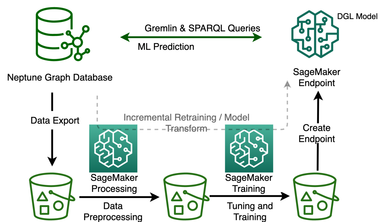
The following figure illustrates different steps for Neptune ML to train a GNN-based recommendation system. Let’s zoom in on each step and explore what it involves:
Data export configuration
The first step in our Neptune ML process is to export the graph data from the Neptune cluster. We must specify the parameters and model configuration for the data export task. We use the Neptune workbench for all of the configurations and commends. The workbench lets us work with the Neptune DB cluster using Jupyter notebooks hosted by Amazon SageMaker. In addition, it provides a number of magic commands in the notebooks that save a great deal of time and effort. Here is our example of export parameters:
In export_params, we must configure the basic setup, such as the Neptune cluster and output Amazon Simple Storage Service (S3) path for exported data storage. The configuration specified in additionalParams is the type of ML task to perform. In this example, link prediction is optionally used to predict a particular edge type (User—FRIEND—User). If no target type is specified, then Neptune ML will assume that the task is Link Prediction. The parameters also specify details about the data stored in our graph and how the ML model will interpret that data (we have “User” as node, and “interests” as node property).
To run each step in the ML building process, simply use Neptune workbench commands. The Neptune workbench contains a line magic and a cell magic that can save you a lot of time managing these steps. To run the data export, use the Neptune workbench command: %neptune_ml export start
Once the export job completes, we will have the Neptune graph exported into CSV format and stored in an S3 bucket. There will be two types of files: nodes.csv and edges.csv. A file named training-data-configuration.json will also be generated which has the configuration needed for Neptune ML to perform model training.
See Export data from Neptune for Neptune ML for more information.
Data preprocessing
Neptune ML performs feature extraction and encoding as part of the data-processing steps. Common types of property pre-processing include: encoding categorical features through one-hot encoding, bucketing numerical features, or using word2vec to encode a string property or other free-form text property values.
In our example, we will simply use the property “interests”. Neptune ML encodes the values as multi-categorical. However, if a categorical value is complex (more than three words per node), then Neptune ML infers the property type to be text and uses the text_word2vec encoding.
To run data preprocessing, use the following Neptune notebook magic command: %neptune_ml dataprocessing start
At the end of this step, a DGL graph is generated from the exported dataset for use by the model training step. Neptune ML automatically tunes the model with Hyperparameter Optimization Tuning jobs defined in training-data-configuration.json. We can download and modify this file to tune the model’s hyperparameters, such as batch-size, num-hidden, num-epochs, dropout, etc. Here is a sample configuration.json file.
See Processing the graph data exported from Neptune for training for more information.
Model training
The next step is the automated training of the GNN model. The model training is done in two stages. The first stage uses a SageMaker Processing job to generate a model training strategy. This is a configuration set that specifies what type of model and model hyperparameter ranges will be used for the model training.
Then, a SageMaker hyperparameter tuning job will be launched. The SageMaker Hyperparameter Tuning Optimization job runs a pre-specified number of model training job trials on the processed data, tries different hyperparameter combinations according to the model-hpo-configuration.json file, and stores the model artifacts generated by the training in the output Amazon S3 location.
To start the training step, you can use the %neptune_ml training start command.
Once all of the training jobs are complete, the Hyperparameter tuning job will save the artifacts from the best performing model, which will be used for inference.
At the end of the training, Neptune ML will instruct SageMaker to save the trained model, the raw embeddings calculated for the nodes and edges, and the mapping information between the embeddings and node indices.
See Training a model using Neptune ML for more information.
Create an inference endpoint in Amazon SageMaker
Now that the graph representation is learned, we can deploy the learned model behind an endpoint to perform inference requests. The model input will be the User for which we need to generate friends’ recommendations, along with the edge type, and the output will be the list of the likely recommended friends for that user.
To deploy the model to the SageMaker endpoint instance, use the %neptune_ml endpoint create command.
Query the ML model using Gremlin
Once the endpoint is ready, we can use it for graph inference queries. Neptune ML supports graph inference queries in Gremlin or SPARQL. In our example, we can now check the friends recommendation with Neptune ML on User “Henry”. It requires nearly the same syntax to traverse the edge, and it lists the other Users that are connected to Henry through the FRIEND connection.
Neptune#ml.prediction returns the connection determined by Neptune ML predictions by using the model that we just trained on the social graph. Bill is returned just like our expectation.
Here is another sample prediction query that is used to predict the top eight users that are most likely to connect with Henry:
The results are ranked from stronger connection to weaker, where link Henry — FRIEND — Colin and Henry — FRIEND — Terry is also proposed. This proposition is through graph-based ML where complex interaction patterns on graph can be explored.
See Gremlin inference queries in Neptune ML for more information.
Model transform or retraining when graph data changes
Another question you might ask is: what if my social network changes, or if I want to make recommendations for newly added users? In these scenarios, where you have continuously changing graphs, you may need to update ML predictions with the newest graph data. The generated model artifacts after training are directly tied to the training graph. This means that the inference endpoint must be updated once the entities in the original training graph changes.
However, you don’t need to retrain the whole model to make predictions on the updated graph. With an incremental model inference workflow, you only need to export the Neptune DB data, perform an incremental data preprocessing, run a model batch transform job, and then update the inference endpoint. The model-transform step takes the trained model from the main workflow and the results of the incremental data preprocessing step as inputs. Then it outputs a new model artifact to use for inference. This new model artifact is created from the up-to-date graph data.
One special focus here is for the model-transform step command. It can compute model artifacts on graph data that was not used for model training. The node embeddings are re-computed and any existing node embeddings are overridden. Neptune ML applies the learned GNN encoder from the previous trained model to the new graph data nodes with their new features. Therefore, the new graph data must be processed using the same feature encodings, and it must adhere to the same graph schema as the original graph data. See more Neptune ML implementation details at Generating new model artifacts.
Moreover, you can retrain the whole model if the graph changes dramatically, or if the previously trained model could no longer accurately represent the underlying interactions. In this case, re-using the learned model parameters on a new graph cannot guarantee a similar model performance. You must retrain your model on the new graph. To accelerate the hyperparameters search, Neptune ML can leverage the information from the previous model training task with warm start: the results of previous training jobs are used to select good combinations of hyperparameters to search over the new tuning job.
See workflows for handling evolving graph data for more details.
Conclusion
In this post, you have seen how Neptune ML and GNNs can help you make recommendations on graph data using a link prediction task by combining information from the complex interaction patterns in the graph.
Link prediction is one way of implementing a recommendation system on graph. You can construct your recommender in many other ways. You can use the embeddings learned during link prediction training to cluster the nodes into different segments in an unsupervised manner, and recommend items to the one belonging to the same segment. Furthermore, you can obtain the embeddings and feed them into a downstream similarity-based recommendation system as an input feature. Now this additional input feature also encodes the semantic information derived from graph and can provide significant improvements to the overall precision of the system. Learn more about Amazon Neptune ML by visiting the website or feel free to ask questions in the comments!
About the Authors
Yanwei Cui, PhD, is a Machine Learning Specialist Solutions Architect at AWS. He started machine learning research at IRISA (Research Institute of Computer Science and Random Systems), and has several years of experience building artificial intelligence powered industrial applications in computer vision, natural language processing and online user behavior prediction. At AWS, he shares the domain expertise and helps customers to unlock business potentials, and to drive actionable outcomes with machine learning at scale. Outside of work, he enjoys reading and traveling.
Will Badr is a Principal AI/ML Specialist SA who works as part of the global Amazon Machine Learning team. Will is passionate about using technology in innovative ways to positively impact the community. In his spare time, he likes to go diving, play soccer and explore the Pacific Islands.
Read MoreAWS Machine Learning Blog