Google Colab for Machine Learning Projects

Last Updated on April 30, 2022

Have you ever wanted an easy-to-configure interactive environment to run your machine learning code that came with access to GPUs for free? Google Colab is the answer you’ve been looking for. It is a convenient and easy to use way to run Jupyter notebooks on the cloud and their free version comes with some limited access to GPUs as well.

If you’re familiar with Jupyter notebooks, learning Colab will be a piece of cake and we can even import Jupyter notebooks to be run on Google Colab. But, there are a lot of nifty things that Colab can do as well, which we’re going to explore in this article. Let’s dive right in!

After completing tutorial, you will learn how to:

Speed up training using Google Colab’s free tier with GPU
Using Google Colab’s extensions to save to Google Drive, present interactive display for pandas DataFrame, etc.
Save your model’s progress when training with Google Colab

Let’s get started!

Overview

This tutorial is divided into 5 parts:

What is Google Colab?
Google Colab quick start guide
Exploring your Colab environment
Useful Google Colab extensions
Example: Saving model progress on Google Drive

What is Google Colab?

From the “Welcome to Colab” notebook,

Colab notebooks allow you to combine executable code and rich text in a single document, along with images, HTML, LaTeX and more. When you create your own Colab notebooks, they are stored in your Google Drive account. You can easily share your Colab notebooks with co-workers or friends, allowing them to comment on your notebooks or even edit them.

We can use Google Colabs like Jupyter notebooks but they are really convenient because they are hosted by Google Colab so we don’t use any of our own compute resources to run the notebook. We can also share these notebooks so other people can easily run our code as well, all with a standard environment since it’s not dependent on our own local machines, though we might need to install some libraries to our environment during initialization.

Google Colab Quick Start Guide

To get create your Google Colab file and get started with Google Colab, you can go to Google Drive and create a Google Drive account if you do not have one. Then, click on the “New” button on the top left corner of your Google Drive page, then click on More ▷ Google Colaboratory.

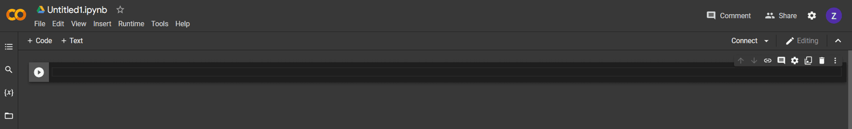
You will then enter the page for your new Google Colab file.

From here, you can share your Google Colab file with others using the Share button on the top right hand corner or start coding!

The hot keys on Colab and that on Jupyter notebooks are similar. These are some of the useful one:

Run cell: Ctrl + Enter
Run cell and add new cell below: Alt + Enter
Run cell and goto cell below: Shift + Enter
Indent line by two spaces: Ctrl + ]
Unindent line by two spaces: Ctrl + [

But there’s also one extra that’s pretty useful that lets you only run a particular selected part of the code in a cell:

Run selected part of a cell: Ctrl + Shift + Enter

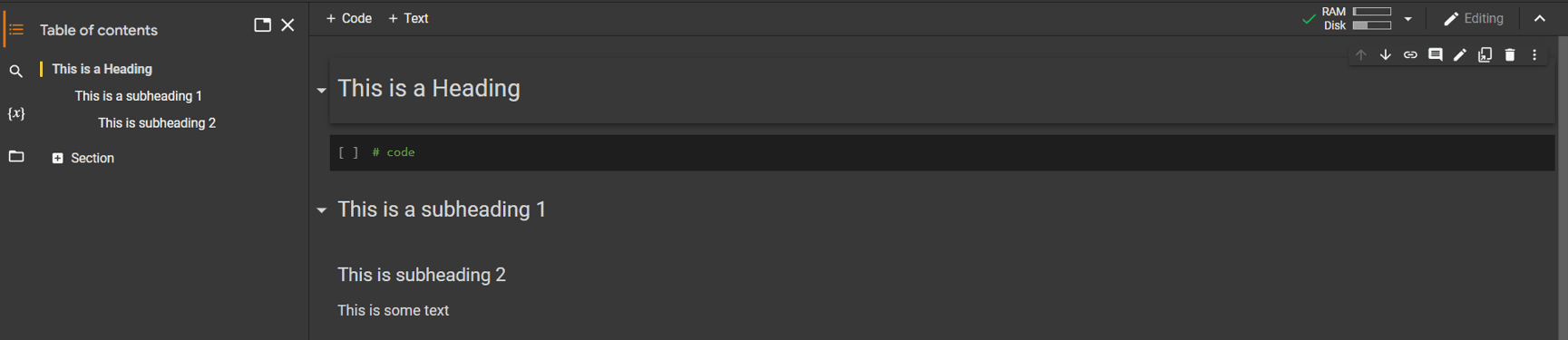
Just like Jupyter notebook, you can also write text with Markdown cells, but Colab has an additional feature that automatically generates a table of contents based on your markdown content and you can also hide parts of the code based on their heading in the markdown cells.

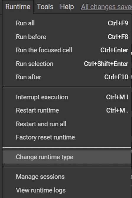
If you run Jupyter on your own computer, you have no choice but use the CPU from your computer. But in Colab, you can change the runtime to include GPUs and TPUs in addition to CPUs, because it is executed on Google’s cloud. You can switch to a different runtime by going to Runtime ▷ Change runtime type:

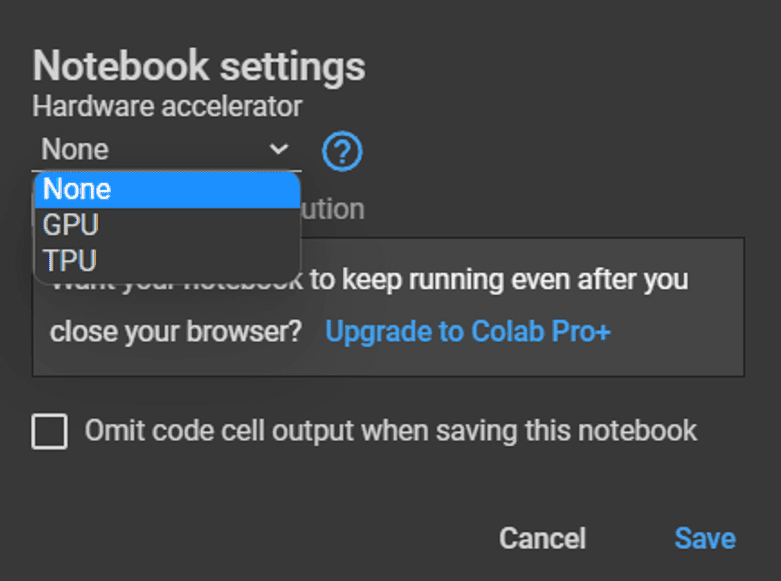
You can then select from the different hardware accelerators to equip your environment with.

Unlike your own computer, Google Colab does not provide you a terminal to enter commands to manage your Python environment. To install Python libraries and other programs, we can use the ! character to run shell commands just like in Jupyter notebooks, e.g. !pip install numpy (but as we’ll see later on, Colab already comes pre-installed with a lot of the libraries we’ll need such as NumPy)

Now that we know how to set up our Colab environment and start running some code, let’s do some exploration of the environment!

Exploring your Colab environment

As we can run some shell command with !, using the wget command is probably the easiest way to get some data. For example, running this will bring you a CSV file to the Colab environment:

! wget https://raw.githubusercontent.com/jbrownlee/Datasets/master/shampoo.csv

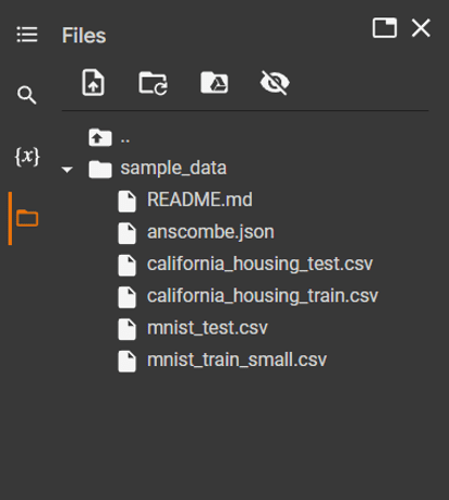
To explore the current working directory of your Colab file on the virtual machine, click on the File icon on the left hand side of the screen. By default, Colab provides you a directory named sample_data with a few files:

This is the current working directory for our Colab notebook. You can read one of these file in Python by using a code like this on the notebook:

file = open(“sample_data/mnist_test.csv”)

Later we’ll see how to use Colab extensions to mount our Google Drive to this directory in order to store and access files on our Google Drive account.

By running shell commands using !, we can also look at the hardware configuration of our Colab environment. To take a look at the CPU, we can use

!cat /proc/cpuinfo

which gave the output for my environment as

processor : 0
vendor_id : GenuineIntel
cpu family : 6
model : 63
model name : Intel(R) Xeon(R) CPU @ 2.30GHz
stepping : 0
microcode : 0x1
cpu MHz : 2299.998
cache size : 46080 KB
…

processor : 1
vendor_id : GenuineIntel
cpu family : 6
model : 63
model name : Intel(R) Xeon(R) CPU @ 2.30GHz
stepping : 0
microcode : 0x1
cpu MHz : 2299.998
cache size : 46080 KB
…

We can also check if we have a GPU attached to the runtime by using

!nvidia-smi

which gave the output if you got one:

+—————————————————————————–+
| NVIDIA-SMI 460.32.03 Driver Version: 460.32.03 CUDA Version: 11.2 |
|——————————-+———————-+———————-+
| GPU Name Persistence-M| Bus-Id Disp.A | Volatile Uncorr. ECC |
| Fan Temp Perf Pwr:Usage/Cap| Memory-Usage | GPU-Util Compute M. |
| | | MIG M. |
|===============================+======================+======================|
| 0 Tesla K80 Off | 00000000:00:04.0 Off | 0 |
| N/A 57C P8 31W / 149W | 0MiB / 11441MiB | 0% Default |
| | | N/A |
+——————————-+———————-+———————-+

+—————————————————————————–+
| Processes: |
| GPU GI CI PID Type Process name GPU Memory |
| ID ID Usage |
|=============================================================================|
| No running processes found |
+—————————————————————————–+

These are just some examples of the shell commands that we can use to explore the Colab environment. There are also many others such as !pip list to look at the libraries which the colab environment has access to, the standard !ls to explore the files in the working directory, etc.

Useful Colab extensions

Colab also comes with a lot of really useful extensions. One such extension allows us to mount our Google Drive to our working directory. We can do this using

import os
from google.colab import drive

MOUNTPOINT = “/content/gdrive”
DATADIR = os.path.join(MOUNTPOINT, “MyDrive”)
drive.mount(MOUNTPOINT)

Then, Colab will request for permission to access your Google Drive files, which you can do after selecting which Google account you want to give it access to. After giving it the required permissions, we can see our Google Drive mounted in the Files tab on the left hand side.

Then, to write a file to our Google Drive, we can do

…
# writes directly to google drive
with open(f”{DATADIR}/test.txt”, “w”) as outfile:
outfile.write(“Hello World!”)

This code snippet writes Hello World! to a test.txt file in the top level of your Google Drive. Similarly, we can read from a file in our Google Drive as well by using:

…
with open(f”{DATADIR}/test.txt”, “r”) as infile:
file_data = infile.read()
print(file_data)

which outputs

Hello World!

based on our earlier example.

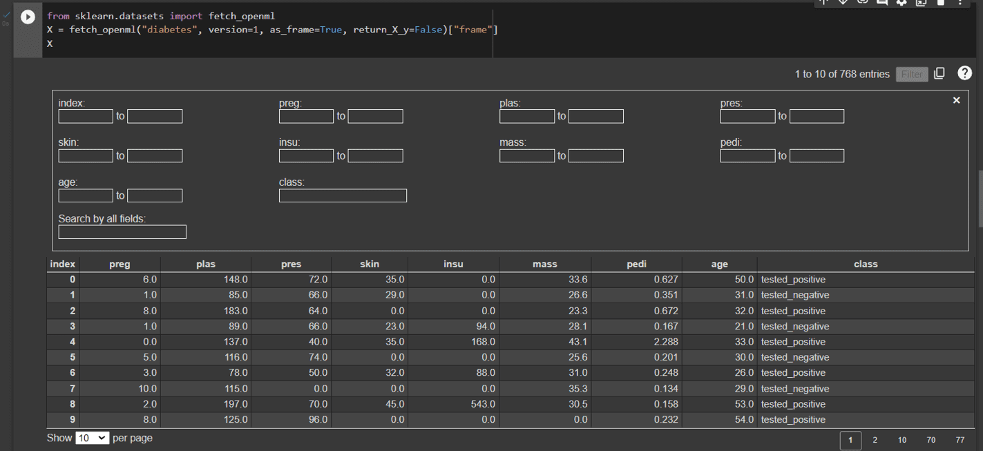
Furthermore, Google Colab comes with some extensions to create better experience on using a notebook. If we use pandas DataFrame a lot, there is an extension to display interactive tables. To use this, we can use magic functions:

%load_ext google.colab.data_table

which enables the interactive display for DataFrames, then when we run

from sklearn.datasets import fetch_openml
X = fetch_openml(“diabetes”, version=1, as_frame=True, return_X_y=False)[“frame”]
X

This will show you the DataFrame as an interactive table, where we can filter based on columns, see the different rows in the table, etc.

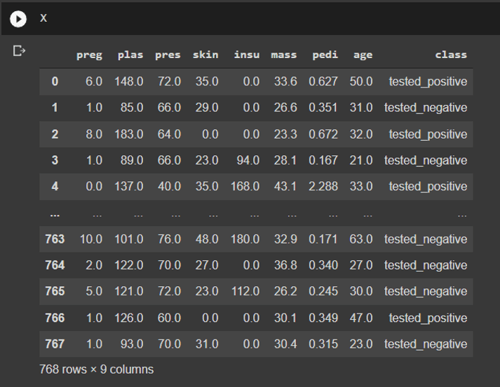
To disable this feature later on, we can run

%unload_ext google.colab.data_table

and when we display the same DataFrame X again, we get the standard Pandas DataFrame interface:

Example: Saving Model Progress on Google Drive

Google Colab is probably the easiest way to give us powerful GPU resources for your machine learning project. But in the free version of Colab, Google limits our time we can use our Colab notebook in each session. Our kernel may terminate for no reason. We can restart our notebook and continue our work, but we may lost everything in the memory. This is a problem if we need to train our model for a long time. Our Colab instance may terminate before the training completed.

Using the Google Colab extension to mount our Google Drive and Keras ModelCheckpoint callback, we are able to save our model progress on Google Drive. This is particularly useful to workaround Colab timeouts. It is more lenient for paid Pro and Pro+ users, but there is always a chance that our model training terminates midway at random times. It is valuable if we don’t lost our partially trained model.

For this demonstration, we’ll use the LeNet-5 model on the MNIST dataset.

import tensorflow as tf
from tensorflow import keras
from keras.layers import Input, Dense, Conv2D, Flatten, MaxPool2D
from keras.models import Model

class LeNet5(tf.keras.Model):
def __init__(self):
super(LeNet5, self).__init__()
#creating layers in initializer
self.conv1 = Conv2D(filters=6, kernel_size=(5,5), padding=”same”, activation=”relu”)
self.max_pool2x2 = MaxPool2D(pool_size=(2,2))
self.conv2 = Conv2D(filters=16, kernel_size=(5,5), padding=”same”, activation=”relu”)
self.flatten = Flatten()
self.fc1 = Dense(units=120, activation=”relu”)
self.fc2 = Dense(units=84, activation=”relu”)
self.fc3=Dense(units=10, activation=”softmax”)
def call(self, input_tensor):
conv1 = self.conv1(input_tensor)
maxpool1 = self.max_pool2x2(conv1)
conv2 = self.conv2(maxpool1)
maxpool2 = self.max_pool2x2(conv2)
flatten = self.flatten(maxpool2)
fc1 = self.fc1(flatten)
fc2 = self.fc2(fc1)
fc3 = self.fc3(fc2)
return fc3

Then, to save model progress during training on Google Drive, first we need to mount our Google Drive onto our Colab environment.

import os
from google.colab import drive
MOUNTPOINT = “/content/gdrive”
DATADIR = os.path.join(MOUNTPOINT, “MyDrive”)
drive.mount(MOUNTPOINT)

Afterwards, we declare the Callback to save our checkpoint model to the Google Drive.

import tensorflow as tf

checkpoint_path = DATADIR + “/checkpoints/cp-epoch-{epoch}.ckpt”
cp_callback = tf.keras.callbacks.ModelCheckpoint(filepath=checkpoint_path,
save_weights_only=True,
verbose=1)

Next, training on the MNIST dataset, with the checkpoint callbacks to ensure we can resume at the last epoch should our Colab session timed out:

import tensorflow as tf
from tensorflow import keras
from keras.layers import Input, Dense, Conv2D, Flatten, MaxPool2D
from keras.models import Model

mnist_digits = keras.datasets.mnist
(train_images, train_labels), (test_images, test_labels) = mnist_digits.load_data()

input_layer = Input(shape=(28,28,1))
model = LeNet5()(input_layer)
model = Model(inputs=input_layer, outputs=model)
model.compile(optimizer=”adam”, loss=tf.keras.losses.SparseCategoricalCrossentropy(), metrics=”acc”)
model.fit(x=train_images, y=train_labels, batch_size=256, validation_data = [test_images, test_labels], epochs=5, callbacks=[cp_callback])

This trains our model and gives the output:

Epoch 1/5
235/235 [==============================] – ETA: 0s – loss: 0.9580 – acc: 0.8367
Epoch 1: saving model to /content/gdrive/MyDrive/checkpoints/cp-epoch-1.ckpt
235/235 [==============================] – 11s 7ms/step – loss: 0.9580 – acc: 0.8367 – val_loss: 0.1672 – val_acc: 0.9492
Epoch 2/5
229/235 [============================>.] – ETA: 0s – loss: 0.1303 – acc: 0.9605
Epoch 2: saving model to /content/gdrive/MyDrive/checkpoints/cp-epoch-2.ckpt
235/235 [==============================] – 1s 5ms/step – loss: 0.1298 – acc: 0.9607 – val_loss: 0.0951 – val_acc: 0.9707
Epoch 3/5
234/235 [============================>.] – ETA: 0s – loss: 0.0810 – acc: 0.9746
Epoch 3: saving model to /content/gdrive/MyDrive/checkpoints/cp-epoch-3.ckpt
235/235 [==============================] – 1s 6ms/step – loss: 0.0811 – acc: 0.9746 – val_loss: 0.0800 – val_acc: 0.9749
Epoch 4/5
230/235 [============================>.] – ETA: 0s – loss: 0.0582 – acc: 0.9818
Epoch 4: saving model to /content/gdrive/MyDrive/checkpoints/cp-epoch-4.ckpt
235/235 [==============================] – 1s 6ms/step – loss: 0.0580 – acc: 0.9819 – val_loss: 0.0653 – val_acc: 0.9806
Epoch 5/5
222/235 [===========================>..] – ETA: 0s – loss: 0.0446 – acc: 0.9858
Epoch 5: saving model to /content/gdrive/MyDrive/checkpoints/cp-epoch-5.ckpt
235/235 [==============================] – 1s 6ms/step – loss: 0.0445 – acc: 0.9859 – val_loss: 0.0583 – val_acc: 0.9825

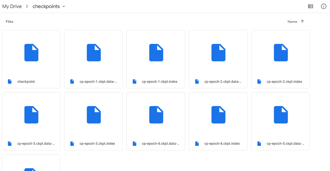
and from the output, we can see that the checkpoints have been saved. Looking at my Google Drive folder, we can also see the checkpoints stored there.

Colab instance is on Google’s cloud environment. The machine it is run has some storage so we can install a package or download some file into it. However, we should not save our checkpoint there because we have no guarantee to get it back after our session terminated. Therefore, in the above, we mount our Google Drive into the instance and save the checkpoint in our Google Drive. This is how we can be assured the checkpoint files are accessible.

Here we attach the full code for the model training and saving to Google Drive:

import os
from google.colab import drive
import tensorflow as tf
from tensorflow import keras
from keras.layers import Input, Dense, Conv2D, Flatten, MaxPool2D
from keras.models import Model

MOUNTPOINT = “/content/gdrive”
DATADIR = os.path.join(MOUNTPOINT, “MyDrive”)
drive.mount(MOUNTPOINT)

class LeNet5(tf.keras.Model):
def __init__(self):
super(LeNet5, self).__init__()
self.conv1 = Conv2D(filters=6, kernel_size=(5,5), padding=”same”, activation=”relu”)
self.max_pool2x2 = MaxPool2D(pool_size=(2,2))
self.conv2 = Conv2D(filters=16, kernel_size=(5,5), padding=”same”, activation=”relu”)
self.flatten = Flatten()
self.fc1 = Dense(units=120, activation=”relu”)
self.fc2 = Dense(units=84, activation=”relu”)
self.fc3=Dense(units=10, activation=”softmax”)
def call(self, input_tensor):
conv1 = self.conv1(input_tensor)
maxpool1 = self.max_pool2x2(conv1)
conv2 = self.conv2(maxpool1)
maxpool2 = self.max_pool2x2(conv2)
flatten = self.flatten(maxpool2)
fc1 = self.fc1(flatten)
fc2 = self.fc2(fc1)
fc3 = self.fc3(fc2)
return fc3

mnist_digits = keras.datasets.mnist
(train_images, train_labels), (test_images, test_labels) = mnist_digits.load_data()

# saving checkpoints
checkpoint_path = DATADIR + “/checkpoints/cp-epoch-{epoch}.ckpt”
cp_callback = tf.keras.callbacks.ModelCheckpoint(filepath=checkpoint_path,
save_weights_only=True,
verbose=1)
input_layer = Input(shape=(28,28,1))
model = LeNet5()(input_layer)
model = Model(inputs=input_layer, outputs=model)
model.compile(optimizer=”adam”, loss=tf.keras.losses.SparseCategoricalCrossentropy(), metrics=”acc”)

model.fit(x=train_images, y=train_labels, batch_size=256, validation_data = [test_images, test_labels],
epochs=5, callbacks=[cp_callback])

If model training stops midway, we can continue by just recompiling the model and loading the weights, and then we can continue our training:

checkpoint_path = DATADIR + “/checkpoints/cp-epoch-{epoch}.ckpt”
cp_callback = tf.keras.callbacks.ModelCheckpoint(filepath=checkpoint_path,
save_weights_only=True,
verbose=1)

input_layer = Input(shape=(28,28,1))
model = LeNet5()(input_layer)
model = Model(inputs=input_layer, outputs=model)
model.compile(optimizer=”adam”, loss=tf.keras.losses.SparseCategoricalCrossentropy(), metrics=”acc”)

# to resume from epoch 5 checkpoints
model.load_weights(DATADIR + “/checkpoints/cp-epoch-5.ckpt”)

# continue training
model.fit(x=train_images, y=train_labels, batch_size=256, validation_data = [test_images, test_labels],
epochs=5, callbacks=[cp_callback])

Further reading

This section provides more resources on the topic if you are looking to go deeper.

Articles

“Welcome to Colab” Notebook: https://colab.research.google.com/
Jupyter Notebook Documentation: https://docs.jupyter.org/en/latest/

Summary

In this tutorial, you have learnt what is Google Colab, how to leverage Google Colab to get free access to GPUs using its free tier, how to use Google Colab with your Google Drive account, and how to save models to store model progress during training on Google Drive in a Google Colab notebook.

Specifically, you learnt:

What is Google Colab and how to start using it
How to explore your Google Colab notebook’s environment using bash commands with !
Useful extensions that come with Google Colab
Saving model progress during training to Google Drive

The post Google Colab for Machine Learning Projects appeared first on Machine Learning Mastery.

Read MoreMachine Learning Mastery