

Customers in industries like consumer packaged goods, manufacturing, and retail are always looking for ways to empower their operational processes by enriching them with insights and analytics generated from data. Tasks like sales forecasting directly affect operations such as raw material planning, procurement, manufacturing, distribution, and inbound/outbound logistics, and it can have many levels of impact, from a single warehouse all the way to large-scale production facilities.
Sales representatives and managers use historical sales data to make informed predictions about future sales trends. Customers use SAP ERP Central Component (ECC) to manage planning for the manufacturing, sale, and distribution of goods. The sales and distribution (SD) module within SAP ECC helps manage sales orders. SAP systems are the primary source of historical sales data.
Sales representatives and managers have the domain knowledge and in-depth understanding of their sales data. However, they lack data science and programming skills to create machine learning (ML) models that can generate sales forecasts. They seek intuitive, simple-to-use tools to create ML models without writing a single line of code.
To help organizations achieve the agility and effectiveness that business analysts seek, we introduced Amazon SageMaker Canvas, a no-code ML solution that helps you accelerate delivery of ML solutions down to hours or days. Canvas enables analysts to easily use available data in data lakes, data warehouses, and operational data stores; build ML models; and use them to make predictions interactively and for batch scoring on bulk datasets—all without writing a single line of code.
In this post, we show how to bring sales order data from SAP ECC to generate sales forecasts using an ML model built using Canvas.
Solution overview
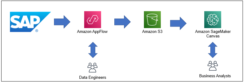
To generate sales forecasts using SAP sales data, we need the collaboration of two personas: data engineers and business analysts (sales representatives and managers). Data engineers are responsible for configuring the data export from the SAP system to Amazon Simple Storage Service (Amazon S3) using Amazon AppFlow, which business analysts can then run either on-demand or automatically (schedule-based) to refresh SAP data in the S3 bucket. Business analysts are then responsible for generating forecasts with the exported data using Canvas. The following diagram illustrates this workflow.
For this post, we use SAP NetWeaver Enterprise Procurement Model (EPM) for the sample data. EPM is generally used for demonstration and testing purposes in SAP. It uses common business process model and follows the business object (BO) paradigm to support a well-defined business logic. We used the SAP transaction SEPM_DG (data generator) to generate around 80,000 historical sales orders and created a HANA CDS view to aggregate the data by product ID, sales date, and city, as shown in the following code:
In the next section, we expose this view using SAP OData services as ABAP structure, which allows us to extract the data with Amazon AppFlow.
The following table shows the representative historical sales data from SAP, which we use in this post.
productid
saledate
city
totalsales
P-4
2013-01-02 00:00:00
Quito
1922.00
P-5
2013-01-02 00:00:00
Santo Domingo
1903.00
The data file is daily frequency historical data. It has four columns (productid, saledate, city, and totalsales). We use Canvas to build an ML model that is used to forecast totalsales for productid in a particular city.
This post has been organized to show the activities and responsibilities for both data engineers and business analysts to generate product sales forecasts.
Data engineer: Extract, transform, and load the dataset from SAP to Amazon S3 with Amazon AppFlow
The first task you perform as a data engineer is to run an extract, transform, and load (ETL) job on historical sales data from SAP ECC to an S3 bucket, which the business analyst uses as the source dataset for their forecasting model. For this, we use Amazon AppFlow, because it provides an out-of-the-box SAP OData Connector for ETL (as shown in the following diagram), with a simple UI to set up everything needed to configure the connection from the SAP ECC to the S3 bucket.
Prerequisites
The following are requirements to integrate Amazon AppFlow with SAP:
SAP NetWeaver Stack version 7.40 SP02 or above
Catalog service (OData v2.0/v2.0) enabled in SAP Gateway for service discovery
Support for client-side pagination and query options for SAP OData Service
HTTPS enabled connection to SAP
Authentication
Amazon AppFlow supports two authentication mechanisms to connect to SAP:
Basic – Authenticates using SAP OData user name and password.
OAuth 2.0 – Uses OAuth 2.0 configuration with an identity provider. OAuth 2.0 must be enabled for OData v2.0/v2.0 services.
Connection
Amazon AppFlow can connect to SAP ECC using a public SAP OData interface or a private connection. A private connection improves data privacy and security by transferring data through the private AWS network instead of the public internet. A private connection uses the VPC endpoint service for the SAP OData instance running in a VPC. The VPC endpoint service must have the Amazon AppFlow service principal appflow.amazonaws.com as an allowed principal and must be available in at least more than 50% of the Availability Zones in an AWS Region.
Set up a flow in Amazon AppFlow
We configure a new flow in Amazon AppFlow to run an ETL job on data from SAP to an S3 bucket. This flow allows for configuration of the SAP OData Connector as source, S3 bucket as destination, OData object selection, data mapping, data validation, and data filtering.
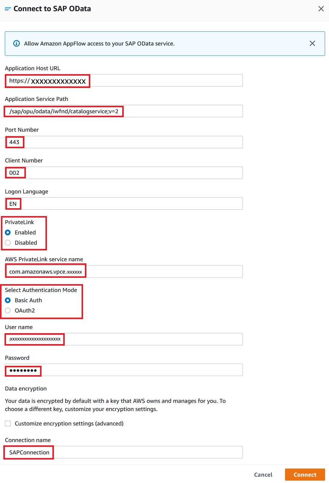
Configure the SAP OData Connector as a data source by providing the following information:
Application host URL
Application service path (catalog path)
Port number
Client number
Logon language
Connection type (private link or public)
Authentication mode
Connection name for the configuration
After you configure the source, choose the OData object and subobject for the sales orders.
Generally, sales data from SAP is exported at a certain frequency, such as monthly or quarterly for the full size. For this post, choose the subobject option for the full-size export.
Choose the S3 bucket as the destination.
The flow exports data to this bucket.
For Data format preference, select CSV format.
For Data transfer preference, select Aggregate all records.
For Filename preference, select Add a timestamp to the file name.
For Folder structure preference, select No timestamped folder.
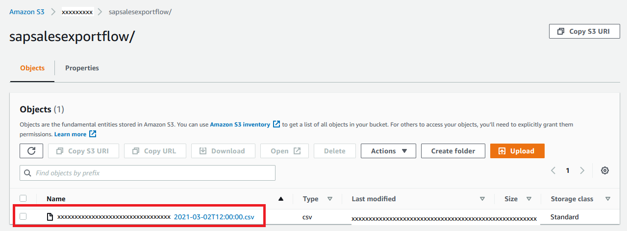
The record aggregation configuration exports the full-size sales data from SAP combined in a single file. The file name ends with a timestamp in the YYYY-MM-DDTHH:mm:ss format in a single folder (flow name) within the S3 bucket. Canvas imports data from this single file for model training and forecasting.
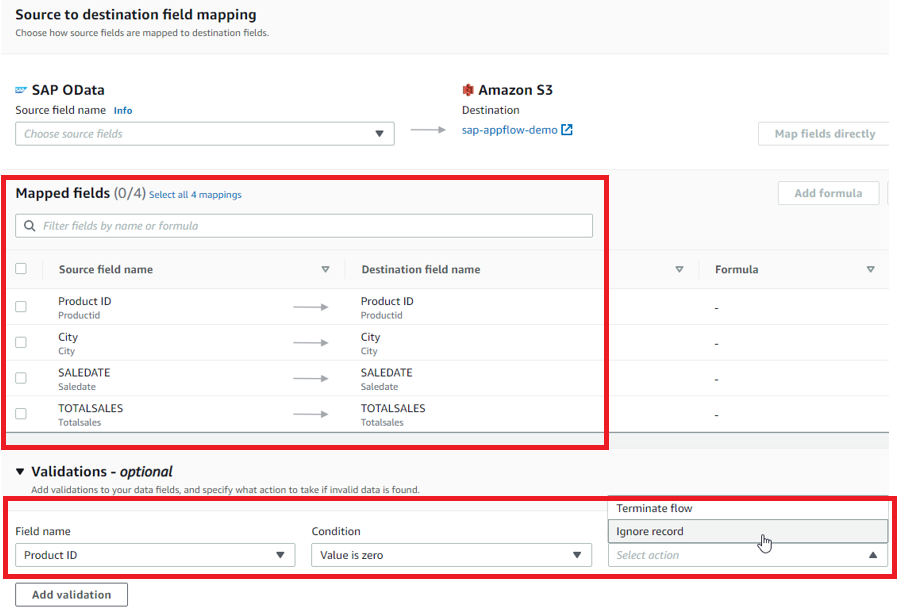
Configure data mapping and validations to map the source data fields to destination data fields, and enable data validation rules as required.
You also configure data filtering conditions to filter out specific records if your requirement demands.
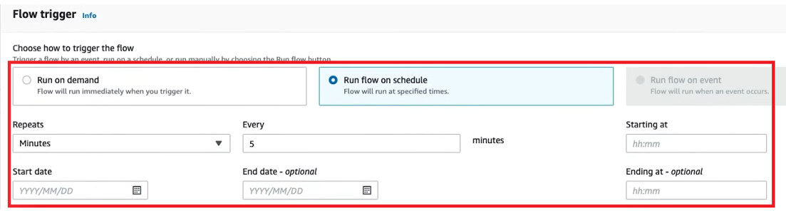
Configure your flow trigger to decide whether the flow runs manually on-demand or automatically based on a schedule.
When configured for a schedule, the frequency is based on how frequently the forecast needs to be generated (generally monthly, quarterly, or half-yearly).
After the flow is configured, the business analysts can run it on demand or based on the schedule to perform an ETL job on the sales order data from SAP to an S3 bucket.
In addition to the Amazon AppFlow configuration, the data engineers also need to configure an AWS Identity and Access Management (IAM) role for Canvas so that it can access other AWS services. For instructions, refer to Give your users permissions to perform time series forecasting.
Business analyst: Use the historical sales data to train a forecasting model
Let’s switch gears and move to the business analyst side. As a business analyst, we’re looking for a visual, point-and-click service that makes it easy to build ML models and generate accurate predictions without writing a single line of code or having ML expertise. Canvas fits the requirement as no-code ML solution.
First, make sure that your IAM role is configured in such a way that Canvas can access other AWS services. For more information, refer to Give your users permissions to perform time series forecasting, or you can ask for help to your Cloud Engineering team.
When the data engineer is done setting up the Amazon AppFlow-based ETL configuration, the historical sales data is available for you in an S3 bucket.
You’re now ready to train a model with Canvas! This typically involves four steps: importing data into the service, configuring the model training by selecting the appropriate model type, training the model, and finally generating forecasts using the model.
Import data in Canvas
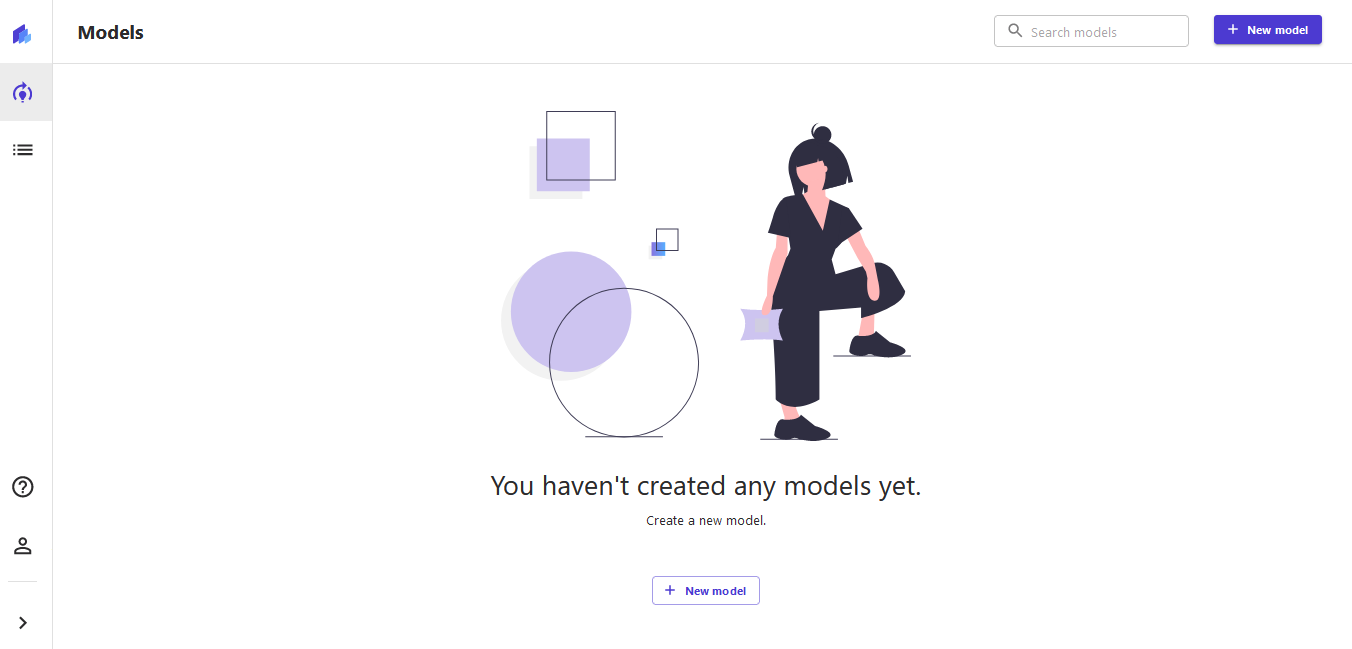
First, launch the Canvas app from the Amazon SageMaker console or from your single sign-on access. If you don’t know how to do that, contact your administrator so that they can guide you through the process of setting up Canvas. Make sure that you access the service in the same Region as the S3 bucket containing the historical dataset from SAP. You should see a screen like the following.
Then complete the following steps:
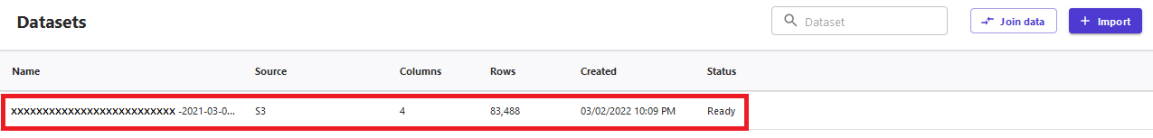
In Canvas, choose Datasets in the navigation pane.
Choose Import to start importing data from the S3 bucket.
On the import screen, choose the data file or object from the S3 bucket to import the training data.
You can import multiple datasets in Canvas. It also supports creating joins between the datasets by choosing Join data, which is particularly useful when the training data is spread across multiple files.
Configure and train the model
After you import the data, complete the following steps:
Choose Models in the navigation pane.
Choose New model to start configuration for training the forecast model.
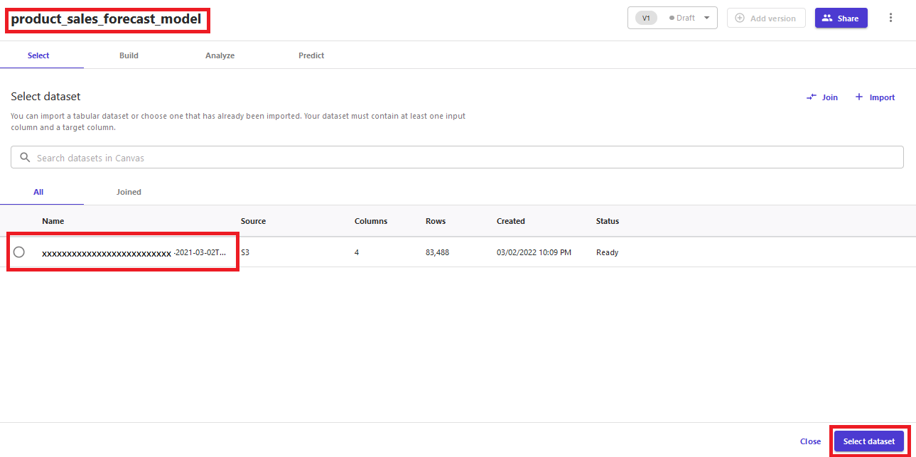
For the new model, give it a suitable name, such as product_sales_forecast_model.
Select the sales dataset and choose Select dataset.
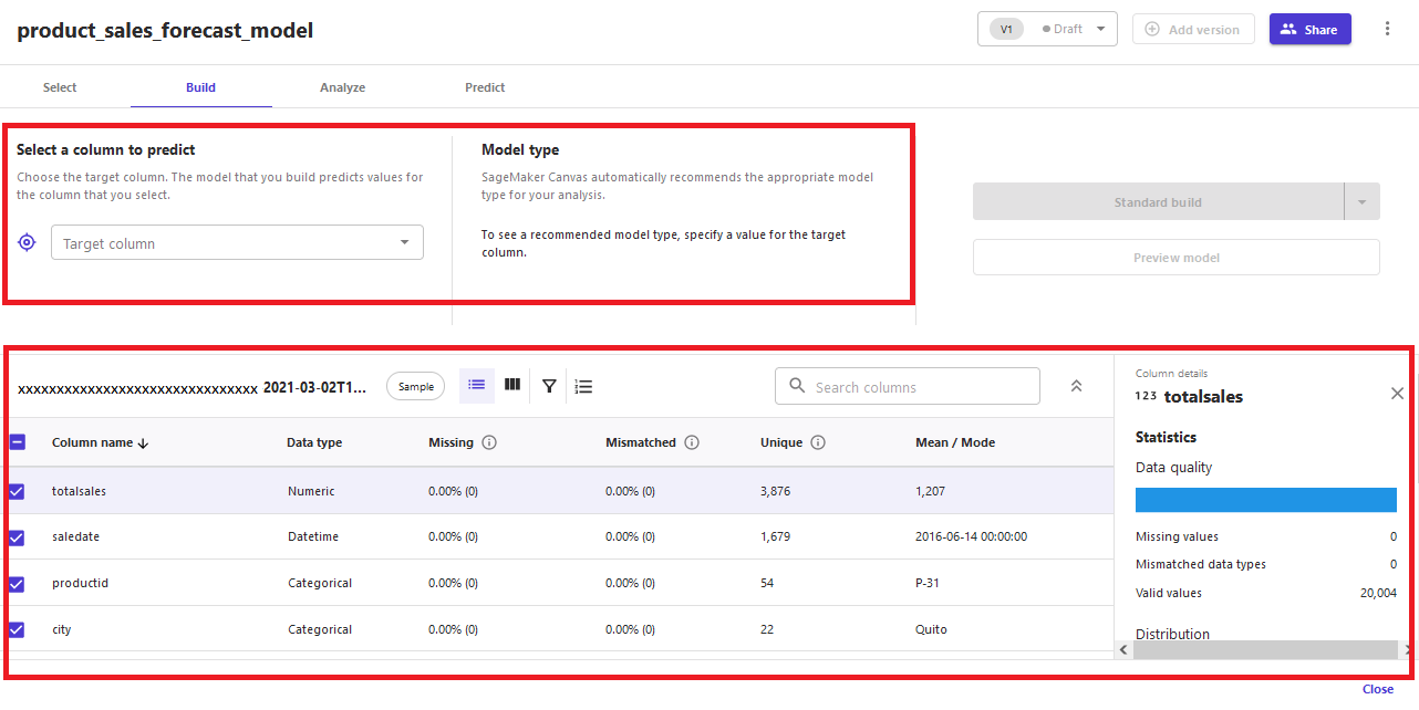
After the dataset is selected, you can see data statistics and configure the model training on the Build tab.
Select totalsales as the target column for the prediction.
You can see Time series forecasting is automatically selected as the model type.
Choose Configure.
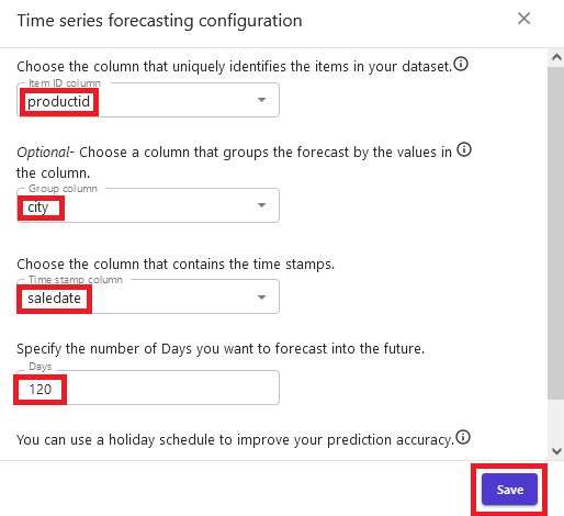
In the Time series forecasting configuration section, choose productid for Item ID column.
Choose city for Group column.
Choose saledate for Time stamp column.
For Days, enter 120.
Choose Save.
This configures the model to make forecasts for totalsales for 120 days using saledate based on historical data, which can be queried for productid and city.
When the model training configuration is complete, choose Standard Build to start the model training.
The Preview model option is not available for time series forecasting model type. You can review the estimated time for the model training on the Analyze tab.
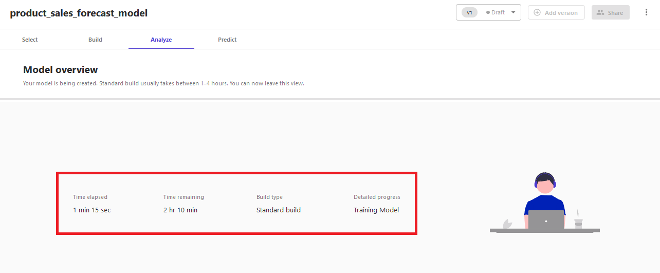
Model training might take 1–4 hours to complete, depending on the data size. When the model is ready, you can use it to generate the forecast.
Generate a forecast
When the model training is complete, it shows prediction accuracy of the model on the Analyze tab. For instance, in this example, it shows prediction accuracy as 92.87%.
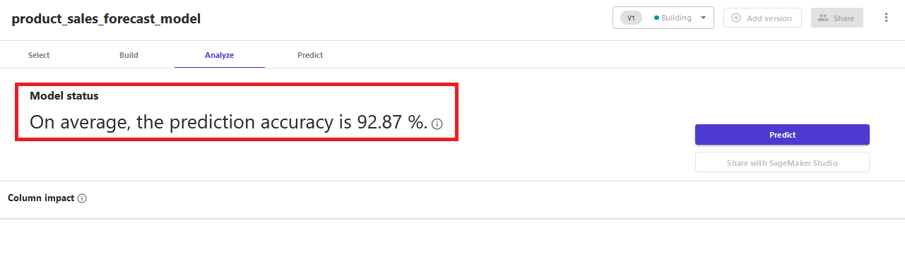
The forecast is generated on the Predict tab. You can generate forecasts for all the items or a selected single item. It also shows the date range for which the forecast can be generated.
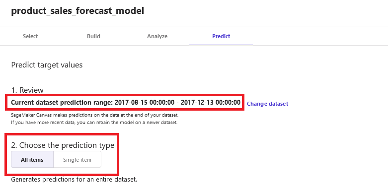
As an example, choose the Single item option. Select P-2 for Item and Quito for Group to generate a prediction for product P-2 for city Quito for the date range 2017-08-15 00:00:00 through 2017-12-13 00:00:00.
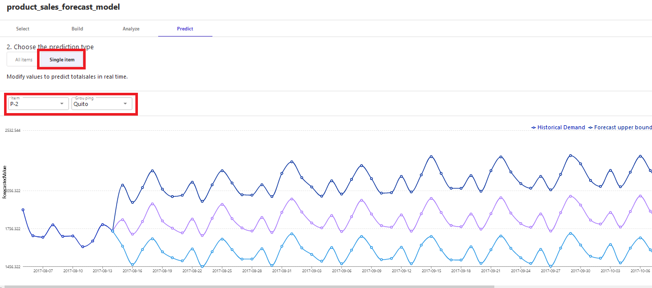
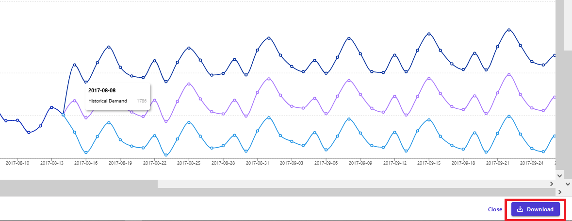
The generated forecast shows the average forecast as well as the upper and lower bound of the forecast. The forecast bounds help configure an aggressive or balanced approach for the forecast handling.
You can also download the generated forecast as a CSV file or image. The generated forecast CSV file is generally to used to work offline with the forecast data.
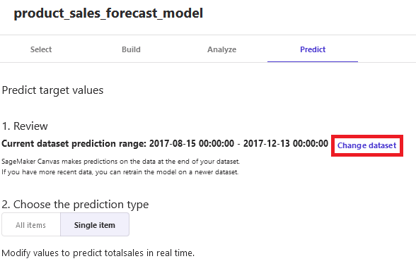
The forecast is now generated for the time series data. When a new baseline of data becomes available for the forecast, you can change the dataset in Canvas to retrain the forecast model using the new baseline.
You can retrain the model multiple times as and when the training data changes.
Conclusion
In this post, you learned how the Amazon AppFlow SAP OData Connector exports sales order data from the SAP system into an S3 bucket and then how to use Canvas to build a model for forecasting.
You can use Canvas for any SAP time series data scenarios, such as expense or revenue prediction. The entire forecast generation process is configuration driven. Sales managers and representatives can generate sales forecasts repeatedly per month or per quarter with a refreshed set of data in a fast, straightforward, and intuitive way without writing a single line of code. This helps improve productivity and enables quick planning and decisions.
To get started, learn more about Canvas and Amazon AppFlow using the following resources:
Amazon SageMaker Canvas Developer Guide
Announcing Amazon SageMaker Canvas – a Visual, No Code Machine Learning Capability for Business Analysts
Extract data from SAP ERP and BW with Amazon AppFlow
SAP OData Connector configuration
About the Authors
Brajendra Singh is solution architect in Amazon Web Services working with enterprise customers. He has strong developer background and is a keen enthusiast for data and machine learning solutions.
Davide Gallitelli is a Specialist Solutions Architect for AI/ML in the EMEA region. He is based in Brussels and works closely with customers throughout Benelux. He has been a developer since he was very young, starting to code at the age of 7. He started learning AI/ML at university, and has fallen in love with it since then.
Read MoreAWS Machine Learning Blog