
 and Amazon Neptune")
A relational database is like a multitool: it can do many things, but it’s not perfectly suited to all tasks. For example, suppose a police department has been using a relational database to perform crime data analysis. As their breadth of sources and volume of data grows, they start to experience performance issues in querying the data. The crime data being ingested is highly connected by nature. Because of its connectedness, in many cases, basic queries involve creating numerous joins over tables containing data such as people, crimes, vehicle registrations, firearm purchases, locations, and persons of interest. Discovering new knowledge and insights is often impossible within the constraints of SQL and the relational table structure. Therefore, they decide that it’s time to utilize a purpose-built database for performing their analysis. Amazon Neptune is a purpose-built, high-performance graph database engine optimized for storing billions of relationships and querying the graph with millisecond latency.
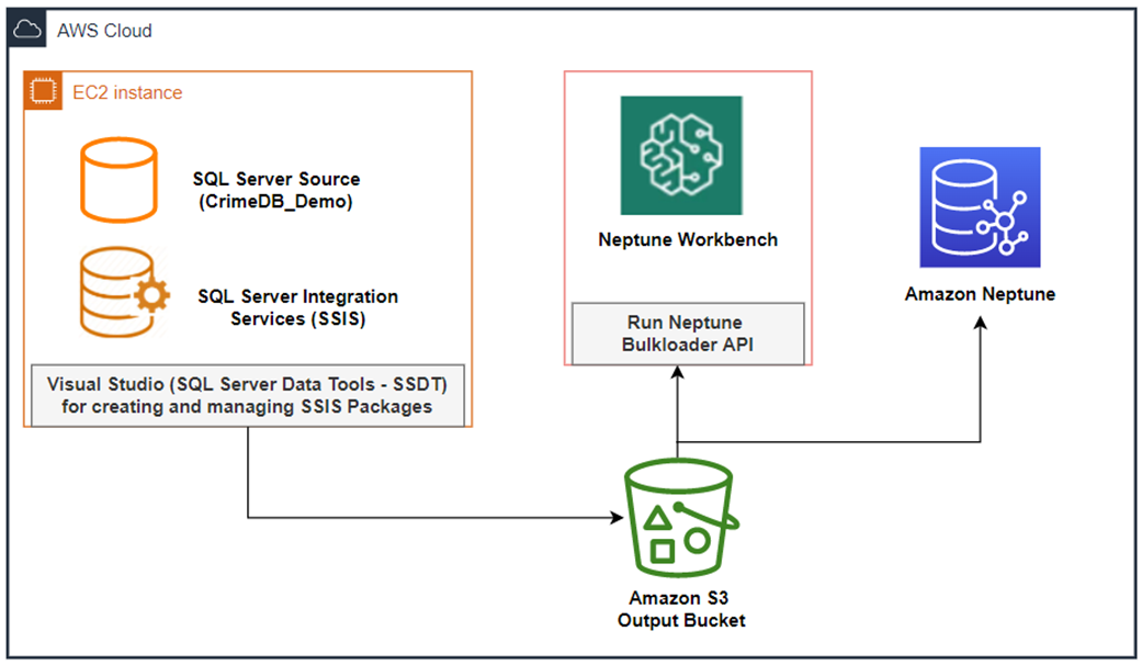
In this post, we describe a solution for this use case to populate a Neptune cluster from your centralized relational database serving as the source of truth while using your current SQL Server Integration Services (SSIS) based extract, transform, and load (ETL) infrastructure. We demonstrate the full data loading process using SSIS and the Neptune Bulk Loader with detailed examples. Although this post specifically demonstrates using SSIS and Neptune Workbench, you can follow the same pattern using other relational databases and ETL tools of your choosing, including AWS Database Migration Service (AWS DMS) or AWS Glue.
Solution overview
We use the following services in our solution:
Amazon Neptune – A fast, reliable, and fully managed graph database service that makes it easy to build and run applications that work with highly connected datasets. It is purpose-built and optimized for storing billions of relationships and querying graph data with millisecond latency.
Neptune Workbench – This workbench lets you work with your DB cluster using Jupyter notebooks hosted by Amazon SageMaker. It provides an interactive query environment where you can issue bulk loads of data into Neptune, explore the data in your DB cluster through queries and visualization, and more.
Amazon S3 – Amazon Simple Storage Service is an object storage service that offers industry-leading scalability, data durability, security, and performance.
SQL Server Integration Services – SSIS is a component of Microsoft SQL Server database software that you can use for performing data extraction, transformation, and loading.
The following diagram shows the architecture of this solution.
The walkthrough includes the following steps:
Set up the target Neptune database and Neptune Workbench.
Set up the source SQL Server database.
Create a destination bucket on Amazon S3.
Convert the dataset from relational to graph and export the dataset to Amazon S3 using SSIS.
Load data from Amazon S3 to Neptune.
Explore data using Neptune Workbench.
Following the walkthrough incurs standard service charges, so you should clean up the resources after completing the exercise.
Prerequisites
This post assumes a working knowledge of SSIS to complete the walkthrough.
Download each of the following sample artifacts:
1-Create DB tables and Insert
2-SSIS ETL Code Initial Load
3-SSIS ETL Code Incremental Load
4-Selecting from the tables-question1
5-Selecting from the tables question2
Crime Sample Notebook
Set up the target Neptune database and Neptune Workbench
First, create a new Neptune cluster. Make sure to select an instance type for the NotebookInstanceType parameter so a Neptune Notebook is spun up with the cluster.
Set up the source SQL Server database
You can create the source database on an existing SQL Server instance you may have on premises or in the cloud. You can also use the AWS Launch Wizard for the guided deployment of a SQL Server instance on Amazon Elastic Compute Cloud (Amazon EC2), which installs a SQL version of your choice along with SSIS.
For this post, an instance of SQL Server 2019 on Microsoft Windows Server 2016 running on Amazon EC2 is used. Make sure to create the instance in the same VPC as the target Neptune cluster. You may use an existing SQL Server Management Studio (SSMS) and SQL Server Data Tool (SSDT) or install both tools on the newly created instance to connect to your database and create your SSIS packages.
When your environment is ready, connect to your SQL Server instance and run the script 1-Create DB tables and Insert.sql to create the sample CrimeDB_Demo database objects and populate the tables with sample data.
All data is for demonstration purposes only and is fictitious by nature; resemblance to actual persons, living or dead, is purely coincidental.
Make sure that the CrimeDB_Demo database and tables have been created successfully. The data in the tables represents mock crime analysis application data, and is designed to allow you to get a feel for how to use a familiar ETL tool (SSIS) for exporting relational data in a graph model that fits the target (Neptune database). You can see the following list of tables after the demo database is created.
Create a destination bucket on Amazon S3
Create an S3 bucket for use as our SSIS package destination and as a source for the Neptune Bulk Loader. For instructions, refer to Create your first S3 bucket.
Convert the dataset from relational to graph
The next step is to convert the relational dataset to a graph data model. Keep in mind the following when planning your data model conversion:
Which graph model to use. Neptune supports both labeled property graphs and the Resource Description Framework.
How to map your relational data to a graph format.
In the following entity-relationship diagram, the CrimeDB_Demo database contains nine tables related with one-to-many and many-to-many relationships. The Crime table holds information about crimes committed. Related details such as the person who committed the crime, the firearm used in the crime, court cases about a specific crime, and so on are stored in their respective tables. When many-to-many relationships occur in the model, you must introduce a JOIN table that holds foreign keys of both the participating tables. For example, the person_crime_Relationship table shows this concept of connecting a person from the Person table to a specific crime in the Crime table by creating a Person-Crime join table containing the ID of the person in one column and the ID of the associated crime in the next column.
Although graph data models don’t require a strict schema like our entity-relationship diagram, different modeling approaches are more effective for particular use cases. Ideally, you’ll work backwards from your business use case, because each graph model type is better suited for answering certain types of questions than others. To understand further considerations to make when transforming from a relational data model to a graph data model, refer to Populating your graph in Amazon Neptune from a relational database using AWS Database Migration Service (DMS) – Part 1: Setting the stage.
For our crime database example, we use the labeled property graph model. In this framework, data is organized into vertices and edges, each of which has a label to categorize similar types of entities into groups. Each vertex and edge can also hold properties (key-value pairs) that describe additional attributes of a particular entity. We’re interested in understanding how different crimes, people, locations, and objects are related to one another, and the property graph model represents our data in an intuitive way. It also makes it easier for us to write traversals based on what attributes a vertex or edge has, and to write questions like “How is person X connected to crime Y?”
To convert our relational table to a property graph model, we map table names to the label of a vertex, with each row in the table corresponding to an individual node with the given label. Each column of the table represents an attribute or property of the translated vertex, and foreign key relationships and the JOIN tables are mapped to edges. Although this is one way to transform from relational to graph, it’s not the only way—for a deeper dive into how to convert models, refer to Populating your graph in Amazon Neptune from a relational database using AWS Database Migration Service (DMS) – Part 2: Designing the property graph model.
With this approach, we can visualize the resulting graph data model as follows.
An abstraction was introduced along the way to condense both vehicles and weapons into one class: Object. This abstraction allows us to write more flexible queries. For example, if we want to write queries that connect to any owned object regardless of if it’s a vehicle or weapon, we can refer to all vertices with a label of Object, then filter by a type attribute if needed. Additionally, by using a more generic label of Object rather than both Vehicle and Weapon, we can add new object types in the future (for example, mobile phones) without having to add more labels.
Create SSIS packages for initial data load
Now that we’ve defined our data model, we can prepare our query to convert our dataset. To do this, you need the following:
Access to the source CrimeDB database
Access to an S3 bucket to store the CSV output
Visual Studio or SQL Server Data Tool (SSDT) with SSIS Powerpack connector (ZappySys installation) or any other SSIS connector that allows Amazon S3 as a destination
For conversion, you can run SQL queries against the source database for use as the data source in the SSIS package. A separate file is created for each node and edges extracted from the relational table. For each select query in the following script, create a separate SSIS package, 2-SSIS ETL Code Initial Load.sql.
To create SSIS packages, complete the following steps:
Open Visual Studio and create a new Integration Services project.
Open the package designer page and enable the data flow task.
From the SSIS Toolbox, drag and drop OLE DB Source and ZS Amazon S3 CSV File Destination into your designer.
Next, you configure the data source information for your relational CrimeDB database.
For Data access mode, select SQL commands and enter the SQL script for each node and edge.
The following screenshots are examples of data sources for exporting the main tables into a graph data model as nodes.
The following screenshots are examples of data sources for exporting relationships into a graph data model as edges.
Configure your Amazon S3 CSV file destination with credentials to your Amazon S3 storage.
Create separate packages for each node and edge, providing an S3 bucket name and file path for each destination file and confirming the input columns to be mapped.
After you create packages for all nodes and edges using the provided SQL command, you will have 10 export packages.
Create a new package with the Execute Package Task that can be used to run the 10 export packages.
Upon completion of SSIS package creation and running all the packages, the S3 bucket should display 10 CSV files (five vertices and five edges) exported by the SSIS package. You can confirm the files were delivered to Amazon S3 via the Amazon S3 console.
Load data from Amazon S3 to Neptune using Neptune Workbench
Now that we have our converted data in Amazon S3, we can bulk load the data files in Amazon S3 into our Neptune cluster. First, open the Neptune Notebook that was deployed with your cluster, and upload the Crime Sample Notebook. This sample notebook contains all of the queries we will be using, so you can follow along with the post.
In the sample notebook, use the %load cell to bulk load the data files. For details on how to use the %load line magic, refer to this guide.
When the full load is complete, validate your data in Neptune with the following queries in separate cells:
Gremlin queries are built via chaining multiple steps together, with the output of one step flowing into the next. In the preceding queries, we collect all the vertices and edges of the graph, then collect the labels for each of those objects, then count how many instances of each label there are.
The results of the queries tell us how many nodes and edges of each label type are present in the graph. We should see the following results:
Before we get started with queries, let’s customize the node icons to make the visualizations more meaningful. We can do tis via the %%graph_notebook_vis_options cell magic in the notebook. Run the following in a notebook cell:
Running this cell lets us specify which icons we want to use to represent nodes of a given label (Person, Location, Object, or Event). We also specify the color of each type of node. To learn about other visualization options that you can adjust through the cell magic, follow along with the sample notebook Grouping-and-Appearance-Customization-Gremlin.ipynb.
Now that we’ve customized our visualization options, let’s get a visual overview of our connected crime data with the following query:
This query gets all the nodes in our graph, traverses to adjacent edges, then traverses onto the connecting node that the traverser did not originate from, and returns the node/edge/node path it took.
In addition of full bulk loading, we could have repeated the same steps described in the full load section to create your packages for the incremental load. The only difference is the scripts you use in the Source Editor, which filters out the newly inserted or modified records since your last incremental load. You can use the sample script 3-SSIS ETL Code Incremental Load.sql to create the data sources for your incremental packages. By utilizing the updatedDate field available in every table, you can filter new records since your previous load.
Query the relational model vs. graph model
Let’s say we want to find everything we have for John Doe II: his address, crimes he was involved in, firearms he owns, vehicles registered to him, and other people who are associated with him. In our relational database, joins are computed at query time by matching primary and foreign keys of all rows in the connected tables. We have to use the foreign key columns in each base table and the lookup tables that establish the many-to-many relationships. To retrieve the records that answer this question, we will have to join six tables, using a sample script 4-Selecting from the tables-question1.sql.
The preceding query returns everything we have about John Doe II, as shown in the following results.
We can also perform this type of query against our knowledge graph. To find information about John Doe II in our graph model, we start by finding the person node that represents him. Then we traverse to the nodes he is immediately connected with, ignoring edge direction. In our Gremlin query, we’re not required to infer connections between entities using unique properties such as foreign keys. Relationships are first-class citizens in a database, so we merely need to find what John Doe II is connected to. See the following code:
We get the following results:
1
{‘zipCode’: [‘22304’], ‘streetAddress’: [‘111 Uline Ave’], ‘city’: [‘Alexandria’], ‘district’: [‘A12’], ‘updatedDate’: [‘2022-04-22 00:00:00’], ‘state’: [‘Virginia’], ‘type’: [‘Address’]}
2
{‘licensePlate’: [‘XY9GD-VA’], ‘color’: [‘Silver’], ‘year’: [‘2016’], ‘vinNumber’: [’39CUFGER0ILU’], ‘model’: [‘G07 X7’], ‘updatedDate’: [‘2022-04-22 00:00:00’], ‘type’: [‘Vehicle’], ‘make’: [‘BMW’]}
3
{‘subtype’: [‘Revolver’], ‘soldBy’: [‘CHESTER CIVILIAN ARMS’], ‘dateSold’: [‘2020-01-12 00:00:00’], ‘updatedDate’: [‘2022-04-22 00:00:00’], ‘type’: [‘Firearm’], ‘category’: [‘Semi-Automatic’]}
4
{‘gender’: [‘Male’], ‘ethnicity’: [‘White’], ‘name’: [‘Carlos Salazar’], ‘updatedDate’: [‘2022-04-22 00:00:00’], ‘age’: [’40’], ‘ssn’: [‘684-85-5446’]}
5
{‘dateOccured’: [‘2020-01-25 00:00:00’], ‘dateReported’: [‘2020-01-25 00:00:00’], ‘updatedDate’: [‘2022-04-22 00:00:00’], ‘type’: [‘Crime’], ‘offenseType’: [‘Child Abduction’]}
6
{‘dateOccured’: [‘2020-07-18 00:00:00’], ‘dateReported’: [‘2020-07-18 00:00:00’], ‘updatedDate’: [‘2022-04-22 00:00:00’], ‘type’: [‘Crime’], ‘offenseType’: [‘Murder’]}
We can also visualize the connections between John Doe II and the nodes he’s connected to with the following query:
We’ve added additional parameters into the Gremlin magic: -l lets us specify the maximum number of characters allowed on a node or edge annotation, and -d lets us specify what annotation should be associated with each node type in the visualization. Before running the preceding query, we ran the following in a separate cell, to denote that the name property should be displayed on nodes of type Person, the type property should be displayed on nodes of type Event and Object, and the streetAddress property should be displayed on nodes of type Location:
The following screenshot shows our generated visualization.
The ability to pre-materialize relationships into the database structure allows graph databases to provide performance above the relational engine, especially for join-heavy queries. By assembling nodes and relationships into connected structures, graph databases enable us to build simple yet sophisticated models that answer our questions.
Of course, if all you’re doing is gathering information about an entity, using a relational database is fine. In our example, we knew what tables we had to join together. But what if we’re looking for insights like “Are these two crimes related?” or “How many connections are between person X and crime Y?” These insights become very difficult to express in a SQL query over a relational schema. The number of joins and self joins are impossible to predict ahead of time. Instead, our graph is much more suited to answer questions like those.
As an example, let’s try to answer the question of how many crimes a person is related to. It’s easy to see if someone is directly related to a crime—from the preceding query, we saw that you can drop in on a person of interest, then make one hop along connected edges to gather all the crimes they’re directly related to. But crime is often more nuanced, where a person may be connected to a crime through another person or object for an unknown number of hops. Let’s see how many people are connected to more than one crime, including connections that may be indirect.
First, we grab all the paths between a person and a crime, even if the person is connected to the crime from more than one hop away:
This query first gathers all the People nodes, then traverses to adjacent nodes across inwards edges, until an Event node is reached. The path of nodes traversed is then returned:
1
path[v[Person-202], v[Event-101]]
2
path[v[Person-203], v[Event-108]]
3
path[v[Person-204], v[Event-107]]
4
path[v[Person-205], v[Event-104]]
…
…
46
path[v[Person-209], v[Person-213], v[Object-809], v[Event-110]]
47
path[v[Person-212], v[Person-207], v[Object-504], v[Event-101]]
48
path[v[Person-214], v[Person-210], v[Object-808], v[Event-110]]
49
path[v[Person-294], v[Person-292], v[Object-891], v[Event-191]]
Going through all the results, you’ll notice that some paths have a direct connection between a person and an event, and some paths have object or person vertices between the starting person and event. This is what we want, because a person might be tied to an event via an object they own, or perhaps they know someone who is directly associated to an event (thereby making themselves indirectly associated). Because we only care about how many different events a person is associated with and not necessarily the specific objects or people that connect them to an event, we need to pull just the person and the event information as pairs from each path. We can do that by adding the following steps to the previous query:
Adding these steps lets us look at each path that was previously found, then create person/event pairs. The final dedup() step removes duplicate pairs that we found. We get the following results:
1
[v[Person-202], v[Event-101]]
2
[v[Person-203], v[Event-108]]
3
[v[Person-204], v[Event-107]]
4
[v[Person-205], v[Event-104]]
…
…
42
[v[Person-209], v[Event-103]]
43
[v[Person-209], v[Event-110]]
44
[v[Person-212], v[Event-101]]
45
[v[Person-214], v[Event-110]]
46
[v[Person-294], v[Event-191]]
Now we have a list of person/event pairs to denote which person is connected to which event, regardless if it’s a direct link to the event or through a number of other person/object connections. Let’s clean this up by grouping the pairs according to which person is represented within the pair, and only including people who are associated with more than one event. We can do this by adding the following steps:
With the steps group().by(limit(local,1)).unfold(), we group each person/event pair by the person within the pair. limit(local,1) collects the first value in our pairs, which is the person of interest. The output of these steps produces the following:
1
{v[Person-291]: [[v[Person-291], v[Event-191]]]}
2
{v[Person-292]: [[v[Person-292], v[Event-191]]]}
3
{v[Person-290]: [[v[Person-290], v[Event-190]]]}
4
{v[Person-295]: [[v[Person-295], v[Event-190]]]}
5
{v[Person-293]: [[v[Person-293], v[Event-190]]]}
…
…
21
{v[Person-208]: [[v[Person-208], v[Event-104]], [v[Person-208], v[Event-110]], [v[Person-208], v[Event-109]]]}
22
{v[Person-209]: [[v[Person-209], v[Event-106]], [v[Person-209], v[Event-103]], [v[Person-209], v[Event-110]]]}
23
{v[Person-206]: [[v[Person-206], v[Event-120]], [v[Person-206], v[Event-102]]]}
24
{v[Person-207]: [[v[Person-207], v[Event-101]]]}
The steps where(select(values).unfold().count().is(gt(1))) keep person/event pairs only if more than one pair is associated with a given person. The output we get from adding these steps produces the following:
1
{v[Person-211]: [[v[Person-211], v[Event-105]], [v[Person-211], v[Event-106]]]}
2
{v[Person-210]: [[v[Person-210], v[Event-108]], [v[Person-210], v[Event-110]]]}
3
{v[Person-221]: [[v[Person-221], v[Event-121]], [v[Person-221], v[Event-120]]]}
4
{v[Person-204]: [[v[Person-204], v[Event-107]], [v[Person-204], v[Event-105]], [v[Person-204], v[Event-102]], [v[Person-204], v[Event-106]]]}
5
{v[Person-215]: [[v[Person-215], v[Event-110]], [v[Person-215], v[Event-109]]]}
…
…
11
{v[Person-208]: [[v[Person-208], v[Event-104]], [v[Person-208], v[Event-110]], [v[Person-208], v[Event-109]]]}
12
{v[Person-209]: [[v[Person-209], v[Event-106]], [v[Person-209], v[Event-103]], [v[Person-209], v[Event-110]]]}
13
{v[Person-206]: [[v[Person-206], v[Event-120]], [v[Person-206], v[Event-102]]]}
Now that we’ve grouped the person/event pairs by person (and filtered the result set to only include people that are associated with more than one event), we can take this a step further and adjust the formatting to make it easier to read. Again, we add the following steps to our query:
The steps order().by(select(values).count(local),decr) orders our list of maps by decreasing the count of unique events .project(‘Person’,’Events’) creates a map with ‘Person’ and ‘Events’ keys, and the respective values of each key are given by the by() statements in the order in which they appear. Therefore, each ‘Person’ key in the map corresponds to the person associated with multiple events (given by select(keys)), and each ‘Events’ key corresponds to the events they’re associated with (given by select(values).unfold().tail(local,1).fold())).
Putting it all together, we have the following query:
We get the following results:
1
{‘Person’: v[Person-205], ‘Events’: [v[Event-104], v[Event-120], v[Event-103], v[Event-122], v[Event-108]]}
2
{‘Person’: v[Person-204], ‘Events’: [v[Event-107], v[Event-105], v[Event-102], v[Event-106]]}
3
{‘Person’: v[Person-202], ‘Events’: [v[Event-101], v[Event-120], v[Event-102]]}
4
{‘Person’: v[Person-214], ‘Events’: [v[Event-105], v[Event-108], v[Event-110]]}
…
…
12
{‘Person’: v[Person-203], ‘Events’: [v[Event-108], v[Event-101]]}
13
{‘Person’: v[Person-206], ‘Events’: [v[Event-120], v[Event-102]]}
It looks like Person-205 is associated (either directly or indirectly) with five different events. Let’s check this out in our graph.
From our earlier view of John Doe II, we observed that he was only directly connected to two crimes. But with our expanded query, we can determine that he is potentially connected to three additional crimes, via his connections through objects he owns and a person he knows.
From the preceding Gremlin query, we learned that we could find the crimes that John Doe II is directly and indirectly related to by making traversals across known connections in our graph. In the relational model, because the information is stored in different tables, to get the same results we must join all the relevant tables to get to the level of possible relationships we need to return. The deeper we go in our hierarchy, the more tables we need to join and the slower our query gets. The example query 5-Selecting from the tables-question2.sql can find the two crimes that John Doe II is directly related to and the three crimes where he is indirectly related.
The following is the result containing all the crimes related to John Doe II, both through direct and indirect relations.
Although we can find similar information using T-SQL, a relational database has limited ability to handle multiple joins, especially on big datasets containing complex relationships. Recursive joins and several nested loop operations on a large number of tables with various levels of relationships can lead to degraded performance.
Clean up your resources
To avoid incurring charges in the future, clean up the resources created as part of the walkthrough in this post:
If you used AWS Launch Wizard to create a new SQL instance, go to AWS Launch Wizard and delete the deployment.
If you used the AWS CloudFormation stack from the instructions Creating a new Neptune DB cluster to create your Neptune cluster and other resources, go to the AWS CloudFormation console and delete the base stack.
If you created the resources manually, make sure you delete all the resources used in this post: the Neptune DB cluster, notebook, S3 buckets, and AWS Identity and Access Management (IAM) user.
Summary
In this post, we demonstrated how to use your existing SQL Server database and SSIS infrastructure to populate and utilize a Neptune graph database optimized to perform queries over highly connected data that is unwieldy and slow, using numerous and recursive joins over a relational database. We showed how to export our existing data using SSIS, load that data into Neptune using the Bulk Loader API, and explore that data using the Neptune Workbench.
Although this post focused on SQL Server and SSIS, you can use the patterns we demonstrated across other relational databases and ETL tools. You can use the examples shown here to improve your existing projects that involve navigating across large, highly connected datasets and when the performance of joining various relational tables can’t keep up with your performance requirements.
Leave any thoughts or questions in the comments section.
About the Authors
Mesgana Gormley is a Senior Database Specialist Solution Architect at Amazon Web Services. She works on the Amazon RDS team providing technical guidance to AWS customers and helping them migrate, design, deploy, and optimize relational database workloads on AWS.
Melissa Kwok is a Neptune Specialist Solutions Architect at AWS, where she helps customers of all sizes and verticals build cloud solutions according to best practices. When she’s not at her desk you can find her in the kitchen experimenting with new recipes or reading a cookbook.
Read MoreAWS Database Blog