

Many AWS customers are looking to solve their business problems by storing and integrating data across a combination of purpose-built databases. The reason for that is purpose-built databases provide innovative ways to build data access patterns that would be challenging or inefficient to solve otherwise. For example, we can model highly connected geospatial data as a graph and store it in Amazon Neptune. We can query such datasets quickly and at massive scale using a graph data model. Another purpose-built database, Amazon OpenSearch Service (successor to Amazon Elasticsearch Service), can store geospatial data and provide powerful geo queries in addition to its full text search capabilities.
For a comprehensive overview of purpose-built databases on AWS, visit Purpose-built databases.
One of the features of Neptune that makes it an attractive option for a wide variety of workloads and access patterns is the ease of integration with other AWS services. For example, we can integrate Neptune with OpenSearch Service by deploying an AWS CloudFormation stack (for more information, visit Amazon Neptune-to-OpenSearch replication setup). In this post, we discuss using Neptune with OpenSearch Service utilizing its geospatial querying capabilities. By combining these purpose-built databases, you can add geospatial query capabilities to popular graph use cases like knowledge graphs, identity graphs, and fraud graphs.
Solution overview
When it comes to building applications that rely on geospatial data, some of the most common customer use cases are as follows:
Given an entity in the dataset, find another entity in that dataset that is located the closest to it on the surface of the earth. For example, given a location of a building, we need to find the nearest building from a given set of building locations.
Given an entity and a geographical radius parameter, find all entities located within this radius of the given entity. For example, given a location of a building and a distance, we need to find all buildings within that radius.
Regarding the first use case, the graph where the entities in question are commonly connected via edges typically doesn’t present computational challenges because the set of the entities eligible for analysis is typically represented by the nodes in the graph directly connected to the starting node.
Answering the second use case is best performed by using a database that has optimized support for geospatial radius query capabilities.
We start with a graph-only solution using Neptune with an Amazon SageMaker notebook to query the graph using Gremlin and demonstrate how to solve the first use case.
In the next step, we look at a solution combining both Neptune and OpenSearch Service using the out-of-the-box integration between both of those data stores, and solve the second use case.
Prerequisites
You need a Neptune cluster to store the geospatial data in graph data model. You also need to provision a managed SageMaker notebook and attach it to the Neptune database cluster.
You can create the Neptune cluster and notebook using the provided CloudFormation template.
Data
Let’s use a fictitious customer, a shipping company that operates multiple distribution centers from where the goods are shipped out to physical brick-and-mortar stores owned or operated by other companies.
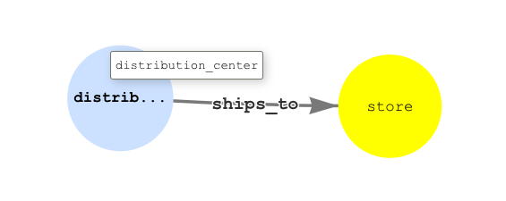
The following graph data model is used to store the distribution centers and stores and the relationship between them.
The distribution_center nodes are connected via optional ships_to edges to the store nodes.
The store nodes have their Neptune ID (T.id, set to correspond to their store ID) and coordinates properties.
The distribution_center nodes have a similar set of properties.
Create synthetic data
Use the following Gremlin query to generate some data and persist it to the graph. Run this query using a Jupyter notebook on SageMaker:
Now you have two distribution_center nodes with four store nodes attached to each one of them via the ships_to edge.
Now that we have loaded our data, let’s look at the solution for the use cases.
Use case 1: Find the nearest stores that a given distribution center ships to
To answer this question, first you need to query the graph, starting at the given distribution_center node, expanding out via the ships_to edges to the store nodes and returning their coordinates.
We use the following Gremlin query:
We get the following result.
Now that you have these nodes’ coordinates properties, you can use the haversine formula (there’s a convenient haversine Python module implementing it) to calculate the distances to see which one is the shortest.
Use the following installation code:
The following is the Python code snippet:
If you iterate over the latitude and longitude values from the result set, you get these distances:
nyc_store_1 – 0.15 miles
nyc_store_2 – 6.8 miles
nyc_store_3 – 13.74 miles
nyc_store_4 – 5.24 miles
After using the Gremlin query and haversine calculation written in Python, you have arrived at the answer to your question: nyc_store_1 is the closest store to distribution_center dc_1.
You can also run the query on the database engine side as opposed to the client side. For more information, visit this guide.
Use case 2: Find store IDs of all stores located within 15 miles of a given distribution center
You can answer this question with Neptune/Gremlin and Python. You can also calculate haversine distances with Gremlin without involving Python, but the unit of work involved in calculating this for a reasonable number of values can get very heavy. For this post, we concentrate on the approach that allows us to split our processing into the traversal step performed by Neptune and the calculation step performed by client-side Python logic.
To answer this question, you need to query all the store nodes in the graph, get their coordinates, calculate the distance from each of these nodes to the distribution center, and compare that distance to a 15-mile constant to see if the store you’re looking at matches our distance criteria.
For the small dataset you have persisted into the graph, this isn’t a problem. In a realistic scenario with thousands of stores, this can become a very expensive workload even when split between Gremlin traversals and Python client-side calculations.
OpenSearch Service has a very handy feature where it can take a set of coordinates and search for entities within a specified radius of these coordinates. Let’s see how you can use that functionality in combination with Neptune to come up with an optimal strategy for the customer’s use case.
Neptune integration with OpenSearch Service
Neptune integrates with OpenSearch Service to support full-text search. This integration uses the Neptune Streams feature to take every change to the graph as it happens, in the order that it is made, and write it to the amazon_neptune index in an OpenSearch Service cluster with a data model (visit Neptune Data Model for OpenSearch Data).
You can use the data in OpenSearch Service for direct querying. In this case, the latitude and longitude can be stored as a geo_point and used for geo queries. This requires updating the default mapping, with a mapping for the graph property that holds the latitude and longitude as comma-separated values.
The following steps enable the geo queries against the graph data synced up to OpenSearch Service:
Enable Neptune integration with OpenSearch Service.
Update OpenSearch Service mapping for the coordinates property.
Load data into the graph.
Run the geo_distance query against the coordinates property.
Prerequisites
For this solution, you should have the following prerequisites:
A Neptune DB cluster with streams enabled
You can use the same Neptune cluster from the previous use case. If you decide to use the same cluster, make sure to clean up the data on it using the gremlin query: g.V().drop()
Follow the instructions in Using Neptune Streams to enable streams
An OpenSearch Service domain
Follow the instructions in Create an OpenSearch Service domain
Enable Neptune integration with OpenSearch Service
Follow the instructions in Amazon Neptune-to-OpenSearch replication setup to configure the integration. The guide walks through the steps of using a prebuilt CloudFormation stack to set up the data synchronization from Neptune to OpenSearch Service.
Update OpenSearch Service mapping
Update the mapping for the coordinates property to geo_point using the OpenSearch Service API:
Load data into the graph
Refer to the step earlier in this post to generate synthetic data using Gremlin. It loads some synthetic data to the graph, and that syncs up that data to OpenSearch.
Run the geo_distance query
Now that you have the data synced up to OpenSearch Service as documents in the amazon_neptune index, you can query OpenSearch Service directly using curl, or programmatically:
We get the following result:
The result of the query shows four stores that are in a 15-mile radius from the NYC distribution center. This shows how OpenSearch Service can perform geo queries on the data ingested from the Neptune graph. In addition to the geo_distance query we demonstrated, OpenSearch Service can do other types of geo queries as well:
geo_bounding_box
geo_polygon
geo_shape
Now you can run Gremlin queries against the graph using the data from the previous OpenSearch Service query. The entity_id field in the OpenSearch Service query results maps to the IDs of the vertices in the graph. Let’s take those entity IDs and query the Neptune graph to retrieve their store ID properties:
We get the following results.
The NYC stores 1, 2, and 3 are in the results because they’re 0.15 miles, 6.8 miles, and 13.74 miles away, respectively, from distribution center dc_1 based on the haversine calculations done in the previous use case. Let’s perform the haversine calculation to find out if nyc_store_4 is indeed within the 15-mile radius.
The coordinates of the store are (40.7128,74.1061):
The calculated haversine distance is 5.2 miles, which means this store node is accurately picked up by the query filtering on a geo distance of 15 miles.
Clean up
To avoid incurring future charges, delete the resources you created as part of this post.
Delete the Cloud Formation stack created for the Neptune to OpenSearch Service integration.
Delete the OpenSearch Service domain.
Delete the Neptune cluster.
Conclusion
In this post, we demonstrated how combining multiple AWS services—in this case Neptune and OpenSearch Service—can help implement solutions for use cases that would be difficult or impossible to address otherwise. We looked at using the haversine formula to manually calculate the distances between the coordinate properties of the nodes, and then expanded our solution to include OpenSearch Service to locate the nodes within a given radius to avoid manual client-side calculations and unnecessarily heavy workloads against Neptune.
If you have any questions or would like to leave feedback, please use the comments section of this post.
About the Authors
Ross Gabay is Senior Database Architect in AWS Professional Services. As the owner of the Neptune Graph DB Practice in ProServe, he works with AWS Customers helping them implement Enterprise-grade solutions using Amazon Neptune and other AWS services.
Abhilash Vinod is a Cloud Application Architect at AWS Professional Services. He helps AWS customers leverage the broad spectrum of services and solutions offered by AWS, to enable innovation and transformation at their businesses.
Read MoreAWS Database Blog