

In the era of Big Data, businesses are faced with a deluge of time series data. This data is not just available in high volumes, but is also highly nuanced. Amazon Forecast Deep Learning algorithms such as DeepAR+ and CNN-QR build representations that effectively capture common trends and patterns across these numerous time series. These algorithms produce forecasts that perform better than traditional forecasting methods.
In some cases, it may be possible to further improve Amazon Forecast accuracy by training the models with similarly behaving subsets of the time series dataset. For example, consider the case of a retail chain. Demand for certain items such as bread and milk is very regular, and likely easy to forecast. In contrast, forecasts for items such as light bulbs, which have intermittent demand, can be difficult to get right. The retailer may also sell sports merchandise for a local team whose demand scales up rapidly leading up to the home games but tapers off soon after. By preprocessing the time series dataset to separate these items into different groups, we give the Amazon Forecast models the ability to learn stronger patterns for the different demand patterns.
In this blog, we’ll learn about one such preprocessing technique called clustering and how it can help you improve your forecasts.
Clustering overview
Clustering is an unsupervised Machine Learning technique that groups items based on some measure of similarity, usually a distance metric. Clustering algorithms seek to split items into groups such that most items within the group are close to each other while being well separated from those in other groups. In the context of time series clustering, Dynamic Time Warping (DTW) is a commonly used distance metric that measures similarity between two sequences based on optimal matching on a non-linear warping path along the time dimension.
This blog post shows you how to preprocess your Target Time Series (TTS) data using K-means algorithm with DTW as the distance metric to produce clusters of homogeneous time series data to train your Amazon Forecast models with. This is an experimental approach and your mileage may vary depending on the composition of your data and expectations around the clustering configuration that best captures its variability. In this demonstration, we set num_clusters=3 with the intention of finding subsets in the time series dataset that correspond to collections of time series that are “smooth”(a very regular distribution of target value over time), “intermittent” (high variations in frequency with relatively consistent target values), and “erratic” (wide variations in both target values and frequency).
The blog post is accompanied by two demo notebooks, the first is optional relating to cleaning of the open source UCI Online Retail II dataset; and the main notebook relating to time series clustering. The dataset comprises of time series data related to business to business online sales of gift-ware in UK over a two-year period. We leverage the tslearn.clustering module of Python tslearn package for clustering of this time series data using DTW Barycenter Averaging (DBA) K-means.
In the following sections, we will dive into the experiment setup and walk through the accompanying notebooks available in the GitHub Clustering Preprocessing notebook repository. The experiment is setup using Jupyter based Python notebooks. Beginner level proficiency in Python and Jupyter/IPython is expected.
(Optional) Data preparation
The optional notebook on Data Cleaning and Preparation processes the UCI Online Retail II dataset and performs a series of data cleaning operations to the columns relevant to this experiment (viz ‘StockCode’, ‘InvoiceDate’ and ‘Quantity’) corresponding to (‘item_id’, ‘timestamp’, ‘target_value’) schema in Amazon Forecast. We roll up the data to daily frequency and resample the time series to fill missing values with zeros. At this stage, we also drop a few time series with unusual stock code data and transpose data to match format needed for clustering.
DBA K-means clustering
Let us begin the discussion on time series clustering with a quick introduction to DTW distances. The DTW algorithm finds a distance between two time series by finding a non-linear, “warped” path along the time dimension that minimizes the cost of matching a pair of time points on the two sequences.
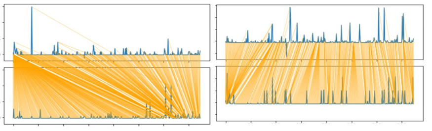
For demonstration, the following plots are generated for the pairs of time series in our dataset. The plot on left presents the DTW path between the first and fifth time series, and the one on the right, between the sixth and tenth time series:
As seen here, matches between the pair of time series are aligned along a warped temporal path (for e.g. time 0th instance of the top-left time series is matched with multiple time points of the bottom left time series, and not strictly t0 to t0, t1 to t1… for the different pairs of time series).
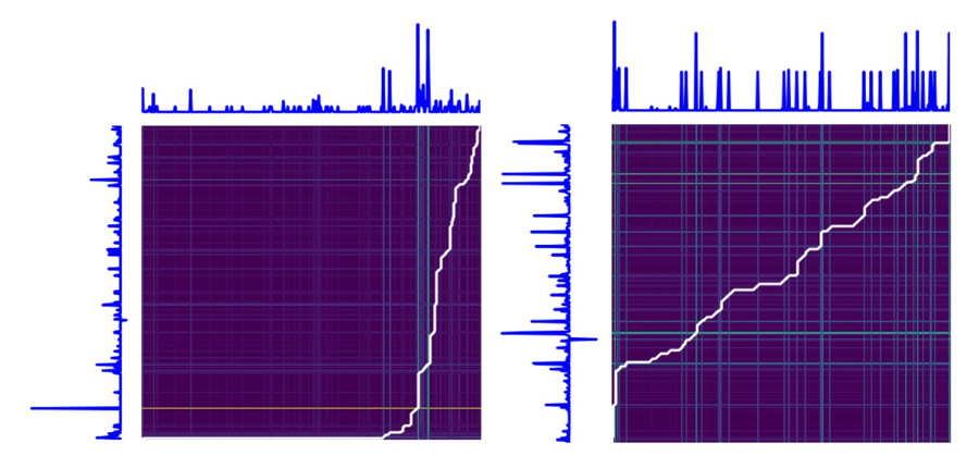
This optimal path is discovered by DTW algorithm by minimizing a suitable metric under a variety of constraints. The following plot demonstrates how DTW algorithm picks the optimal path (represented in white) based on the cost matrix of matching the two pairs of time series from the preceding example. We notice for the left plot that t0 of time series along Y axis gets matched with many time points of time series along axis X, an exact replica of the warped path from the preceding plots:
In the Time Series Clustering notebook, we will train a K-means Clustering algorithm based on DTW distance with Barycenter Averaging. First, we convert the dataframe to tslearn time_series_dataset object and normalize the time series to zero mean and unit variance. We then train the TimeSeriesKMeans method from tslearn.clustering module applying the follow clustering configuration:
n_jobs=-1 ensures that the training uses all available cores on your machine. On a machine with 12 cores (CPU), training the clustering model took roughly half an hour of wall time. Your mileage may vary depending on your machine’s configuration. Other alternative to the distance metric is “softdtw” which may at times produce improved separation, at a higher compute cost.
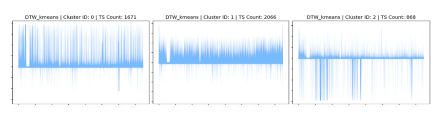
Following figure provide a visual representation of the composition of different clusters discovered by DBA K-means algorithm and corresponding counts of constituent time series (which add up to the overall count of time series in the un-clustered dataset). This representation also gives a good sense of the consistency of the different clusters as the component time series signals are plotted all together, in an overlapping fashion:
You may also notice that the data range is bounded. This is due to the preceding normalizing step that allows for comparisons in an amplitude invariant manner. On closer inspection, we find that individual cluster composition is homogeneous, and the distribution of time series by clusters is balanced (roughly in the proportion 4:5:2).
With the clusters identified, we now split the TTS into subsets based on the labels for the different time series in the dataset. We also reformat the data from columnar time to indexed time to match schema consistent with the Amazon Forecast service APIs. These TTS files are now ready to be used to train Amazon Forecast models.
Results
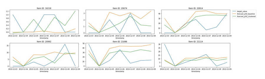
In the following plots, we present a comparison between the baseline (all data taken together), and clustered approach (num_clusters=3) where we split the dataset and train AutoML models for each cluster separately. The following plots are for a few representative samples and compare p50 forecasts obtained from these models for one week worth of hold out set data that the models have not seen previously:
As seen here, the green line, representing the clustered data forecast appears to track the actual target values from the hold out set (in blue) slightly better than the baseline (in orange) model trained with all data together.
As risk of over-fitting exists with very high cluster counts, we recommend setting num_clusters=3 as we have found this setting to work well in experiments with real world datasets, which usually have a mixture of regular, intermittent and otherwise lumpy demand. If you have observed a lot more variety to exist in your dataset, you may choose a more appropriate value for this parameter based on your experience. Also, clustering techniques are not advised for datasets with fewer than a thousand time series since splitting the dataset could have limiting effect on Deep Learning models that thrive on large volumes of data.
Conclusion
Clustering can be a valuable addition to your target time series data preprocessing pipeline. Once the Clustering preprocessing is complete, you may train multiple Amazon Forecast models for the different clusters of the TTS data, or decide to include the clustering configuration as item metadata for the overall TTS. You will find the Forecast Developers Guide helpful for data ingestion, predictor training and generating forecasts. If you have item metadata (IM) and related time series (RTS) data, you can also include those in Amazon Forecast training as previously. Happy Experimenting!
References
Dua, D. and Graff, C. (2019). UCI Machine Learning Repository [http://archive.ics.uci.edu/ml]. Irvine, CA: University of California, School of Information and Computer Science.
Link to UCI Online Retail II dataset repository: https://archive.ics.uci.edu/ml/datasets/Online+Retail+II
Link to UCI Online Retail II dataset: https://archive.ics.uci.edu/ml/machine-learning-databases/00502/online_retail_II.xlsx
Link to tslearn GitHub repository: https://github.com/tslearn-team/tslearn
About the Authors
Vivek M Agrawal is a Data Scientist on the Amazon Forecast team. Over the years, he has applied his passion for Machine Learning to help customers build cutting edge AI/ML solutions in the Cloud. In his free time, he enjoys exploring different cuisines, documentaries, and playing board games.
Read MoreAWS Machine Learning Blog