A Gentle Introduction to the Laplacian

Last Updated on August 6, 2021

The Laplace operator was first applied to the study of celestial mechanics, or the motion of objects in outer space, by Pierre-Simon de Laplace, and as such has been named after him. 

The Laplace operator has since been used to describe many different phenomena, from electric potentials, to the diffusion equation for heat and fluid flow, and quantum mechanics. It has also been recasted to the discrete space, where it has been used in applications related to image processing and spectral clustering. 

In this tutorial, you will discover a gentle introduction to the Laplacian. 

After completing this tutorial, you will know:

The definition of the Laplace operator and how it relates to divergence.
How the Laplace operator relates to the Hessian. 
How the continuous Laplace operator has been recasted to discrete-space, and applied to image processing and spectral clustering. 

Let’s get started. 

Tutorial Overview

This tutorial is divided into two parts; they are:

The Laplacian
The Concept of Divergence
The Continuous Laplacian

The Discrete Laplacian

Prerequisites

For this tutorial, we assume that you already know what are:

The gradient of a function
Higher-order derivatives
Multivariate functions
The Hessian matrix

You can review these concepts by clicking on the links given above.

The Laplacian

The Laplace operator (or Laplacian, as it is often called) is the divergence of the gradient of a function. 

In order to comprehend the previous statement better, it is best that we start by understanding the concept of divergence. 

The Concept of Divergence

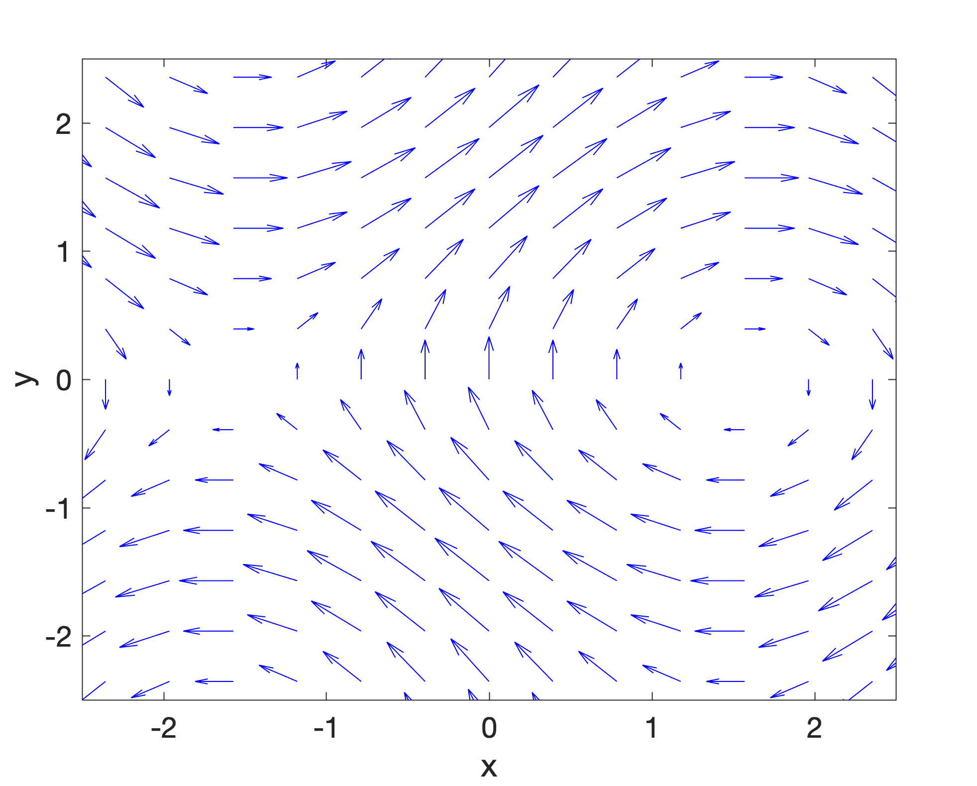
Divergence is a vector operator that operates on a vector field. The latter can be thought of as representing a flow of a liquid or gas, where each vector in the vector field represents a velocity vector of the moving fluid. 

Roughly speaking, divergence measures the tendency of the fluid to collect or disperse at a point …

– Page 432, Single and Multivariable Calculus, 2020.

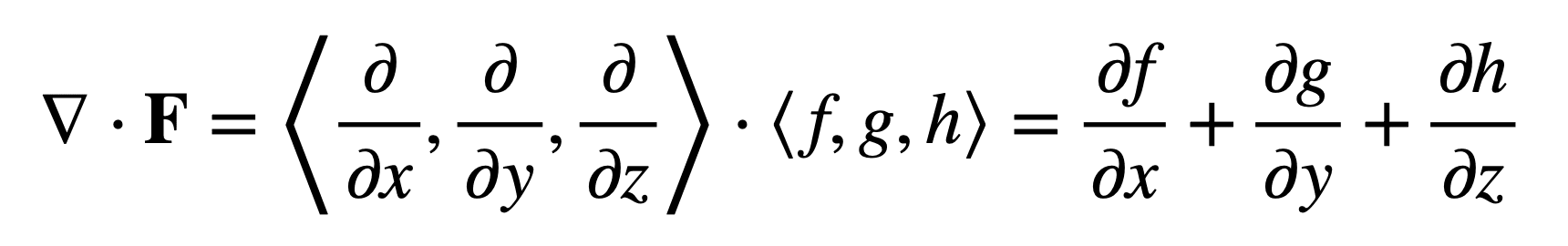
Using the nabla (or del) operator, ∇, the divergence is denoted by ∇ . and produces a scalar value when applied to a vector field, measuring the quantity of fluid at each point. In Cartesian coordinates, the divergence of a vector field, F = ⟨f, g, h⟩, is given by:

Although the divergence computation involves the application of the divergence operator (rather than a multiplication operation), the dot in its notation is reminiscent of the dot product, which involves the multiplication of the components of two equal-length sequences (in this case, ∇ and F) and the summation of the resulting terms. 

The Continuous Laplacian

Let’s return back to the definition of the Laplacian. 

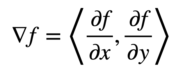
Recall that the gradient of a two-dimensional function, f,  is given by:

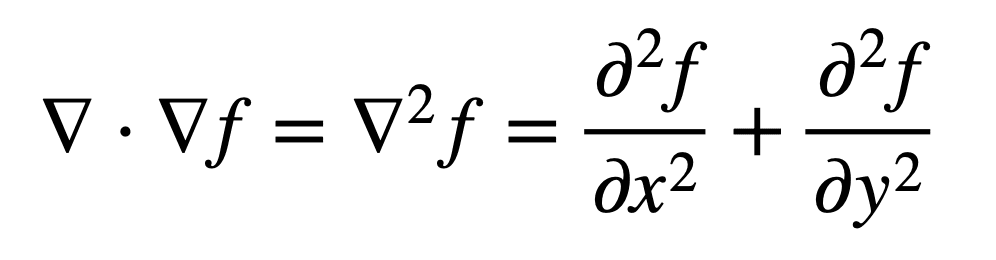
Then, the Laplacian (that is, the divergence of the gradient) of f can be defined by the sum of unmixed second partial derivatives:

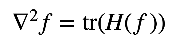
It can, equivalently, be considered as the trace (tr) of the function’s Hessian, H(f). The trace defines the sum of the elements on the main diagonal of a square n×n matrix, which in this case is the Hessian, and also the sum of its eigenvalues. Recall that the Hessian matrix contains the own (or unmixed) second partial derivatives on the diagonal:

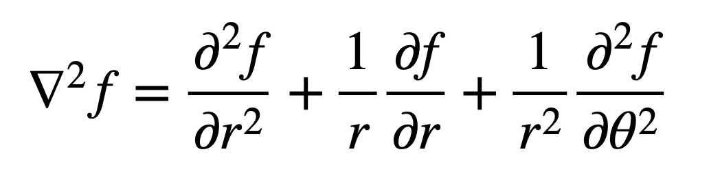
An important property of the trace of a matrix is its invariance to a change of basis. We have already defined the Laplacian in Cartesian coordinates. In polar coordinates, we would define it as follows:

The invariance of the trace to a change of basis means that the Laplacian can be defined in different coordinate spaces, but it would give the same value at some point (x, y) in the Cartesian coordinate space, and at the same point (r, θ) in the polar coordinate space. 

Recall that we had also mentioned that the second derivative can provide us with information regarding the curvature of a function. Hence, intuitively, we can consider the Laplacian to also provide us with information regarding the local curvature of a function, through this summation of second derivatives.

The continuous Laplace operator has been used to describe many physical phenomena, such as electric potentials, and the diffusion equation for heat flow. 

The Discrete Laplacian

Analogous to the continuous Laplace operator, is the discrete one, so formulated in order to be applied to a discrete grid of, say, pixel values in an image, or to a graph. 

Let’s have a look at how the Laplace operator can be recasted for both applications. 

In image processing, the Laplace operator is realized in the form of a digital filter that, when applied to an image, can be used for edge detection. In a sense, we can consider the Laplacian operator used in image processing to, also, provide us with information regarding the manner in which the function curves (or bends) at some particular point, (x, y). 

In this case, the discrete Laplacian operator (or filter) is constructed by combining two, one-dimensional second derivative filters, into a single two-dimensional one:

In machine learning, the information provided by the discrete Laplace operator as derived from a graph can be used for the purpose of data clustering.

Consider a graph, G = (V, E), having a finite number of V vertices and E edges. Its Laplacian matrix, L, can be defined in terms of the degree matrix, D, containing information about the connectivity of each vertex, and the adjacency matrix, A, which indicates pairs of vertices that are adjacent in the graph:

L = D – A

Spectral clustering can be carried out by applying some standard clustering method (such as k-means) on the eigenvectors of the Laplacian matrix, hence partitioning the graph nodes (or the data points) into subsets. 

One issue that can arise in doing so relates to a problem of scalability with large datasets, where the eigen-decomposition (or the extraction of the eigenvectors) of the Laplacian matrix may be prohibitive. The use of deep learning has been proposed to address this problem, where a deep neural network is trained such that its outputs approximate the eigenvectors of the graph Laplacian. The neural network, in this case, is trained using a constrained optimization approach, to enforce the orthogonality of the network outputs. 

Further Reading

This section provides more resources on the topic if you are looking to go deeper.

Books

Single and Multivariable Calculus, 2020.
Handbook of Image and Video Processing, 2005. 

Articles

Laplace operator, Wikipedia. 
Divergence, Wikipedia. 
Discrete Laplace operator, Wikipedia.
Laplacian matrix, Wikipedia. 
Spectral clustering, Wikipedia. 

Papers

SpectralNet: Spectral Clustering Using Deep Neural Networks, 2018.

Summary

In this tutorial, you discovered a gentle introduction to the Laplacian. 

Specifically, you learned:

The definition of the Laplace operator and how it relates to divergence.
How the Laplace operator relates to the Hessian. 
How the continuous Laplace operator has been recasted to discrete-space, and applied to image processing and spectral clustering.

Do you have any questions?
Ask your questions in the comments below and I will do my best to answer.

The post A Gentle Introduction to the Laplacian appeared first on Machine Learning Mastery.

Read MoreMachine Learning Mastery