

Gradient descent procedure is a method that holds paramount importance in machine learning. It is often used for minimizing error functions in classification and regression problems. It is also used in training neural networks, and deep learning architectures.
In this tutorial, you will discover the gradient descent procedure.
After completing this tutorial, you will know:
Gradient descent method
Importance of gradient descent in machine learning
Let’s get started.
Tutorial Overview
This tutorial is divided into two parts; they are:
Gradient descent procedure
Solved example of gradient descent procedure
Prerequisites
For this tutorial the prerequisite knowledge of the following topics is assumed:
A function of several variables
Partial derivatives and gradient vectors
You can review these concepts by clicking on the link given above.
Gradient Descent Procedure
The gradient descent procedure is an algorithm for finding the minimum of a function.
Suppose we have a function f(x), where x is a tuple of several variables,i.e., x = (x_1, x_2, …x_n). Also, suppose that the gradient of f(x) is given by ∇f(x). We want to find the value of the variables (x_1, x_2, …x_n) that give us the minimum of the function. At any iteration t, we’ll denote the value of the tuple x by x[t]. So x[t][1] is the value of x_1 at iteration t, x[t][2] is the value of x_2 at iteration t, e.t.c.
The Notation
We have the following variables:
t = Iteration number
T = Total iterations
n = Total variables in the domain of f (also called the dimensionality of x)
j = Iterator for variable number, e.g., x_j represents the jth variable
𝜂 = Learning rate
∇f(x[t]) = Value of the gradient vector of f at iteration t
The Training Method
The steps for the gradient descent algorithm are given below. This is also called the training method.
Choose a random initial point x_initial and set x[0] = x_initial
For iterations t=1..T
Update x[t] = x[t-1] – 𝜂∇f(x[t-1])
It is as simple as that!
The learning rate 𝜂 is a user defined variable for the gradient descent procedure. Its value lies in the range [0,1].
The above method says that at each iteration we have to update the value of x by taking a small step in the direction of the negative of the gradient vector. If 𝜂=0, then there will be no change in x. If 𝜂=1, then it is like taking a large step in the direction of the negative of the gradient of the vector. Normally, 𝜂 is set to a small value like 0.05 or 0.1. It can also be variable during the training procedure. So your algorithm can start with a large value (e.g. 0.8) and then reduce it to smaller values.
Example of Gradient Descent
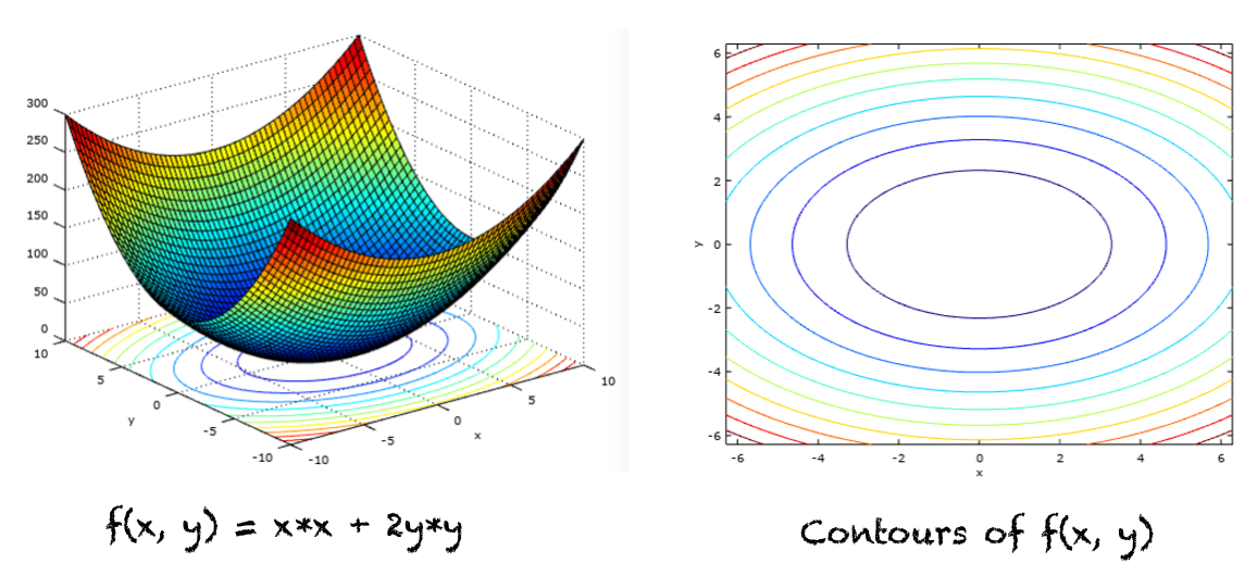
Let’s find the minimum of the following function of two variables, whose graphs and contours are shown in the figure below:
f(x,y) = x*x + 2y*y
The general form of the gradient vector is given by:
∇f(x,y) = 2xi + 4yj
Two iterations of the algorithm, T=2 and 𝜂=0.1 are shown below
Initial t=0
x[0] = (4,3) # This is just a randomly chosen point
At t = 1
x[1] = x[0] – 𝜂∇f(x[0])
x[1] = (4,3) – 0.1*(8,12)
x[1] = (3.2,1.8)
At t=2
x[2] = x[1] – 𝜂∇f(x[1])
x[2] = (3.2,1.8) – 0.1*(6.4,7.2)
x[2] = (2.56,1.08)
If you keep running the above iterations, the procedure will eventually end up at the point where the function is minimum, i.e., (0,0).
At iteration t=1, the algorithm is illustrated in the figure below:
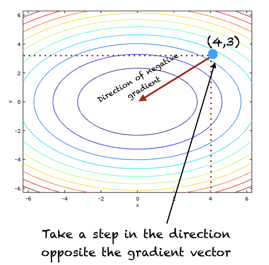
How Many Iterations to Run?
Normally gradient descent is run till the value of x does not change or the change in x is below a certain threshold. The stopping criterion can also be a user defined maximum number of iterations (that we defined earlier as T).
Adding Momentum
Gradient descent can run into problems such as:
Oscillate between two or more points
Get trapped in a local minimum
Overshoot and miss the minimum point
To take care of the above problems, a momentum term can be added to the update equation of gradient descent algorithm as:
x[t] = x[t-1] – 𝜂∇f(x[t-1]) + 𝛼*Δx[t-1]
where Δx[t-1] represents the change in x, i.e.,
Δx[t] = x[t] – x[t-1]
The initial change at t=0 is a zero vector. For this problem Δx[0] = (0,0).
About Gradient Ascent
There is a related gradient ascent procedure, which finds the maximum of a function. In gradient descent we follow the direction of the rate of maximum decrease of a function. It is the direction of the negative gradient vector. Whereas, in gradient ascent we follow the direction of maximum rate of increase of a function, which is the direction pointed to by the positive gradient vector. We can also write a maximization problem in terms of a maximization problem by adding a negative sign to f(x), i.e.,
maximize f(x) w.r.t x is equivalent to minimize -f(x) w.r.t x
Why Is The Gradient Descent Important In Machine Learning?
The gradient descent algorithm is often employed in machine learning problems. In many classification and regression tasks, the mean square error function is used to fit a model to the data. The gradient descent procedure is used to identify the optimal model parameters that lead to the lowest mean square error.
Gradient ascent is used similarly, for problems that involve maximizing a function.
Extensions
This section lists some ideas for extending the tutorial that you may wish to explore.
Hessian matrix
Jacobian
If you explore any of these extensions, I’d love to know. Post your findings in the comments below.
Further Reading
This section provides more resources on the topic if you are looking to go deeper.
Tutorials
Derivatives
Slopes and tangents
Gradient descent for machine learning
What is gradient in machine learning
Partial derivatives and gradient vectors
Resources
Additional resources on Calculus Books for Machine Learning
Books
Thomas’ Calculus, 14th edition, 2017. (based on the original works of George B. Thomas, revised by Joel Hass, Christopher Heil, Maurice Weir)
Calculus, 3rd Edition, 2017. (Gilbert Strang)
Calculus, 8th edition, 2015. (James Stewart)
Summary
In this tutorial, you discovered the algorithm for gradient descent. Specifically, you learned:
Gradient descent procedure
How to apply gradient descent procedure to find the minimum of a function
How to transform a maximization problem into a minimization problem
Do you have any questions?
Ask your questions in the comments below and I will do my best to answer.
The post A Gentle Introduction To Gradient Descent Procedure appeared first on Machine Learning Mastery.
Read MoreMachine Learning Mastery