The Chain Rule of Calculus for Univariate and Multivariate Functions

The chain rule allows us to find the derivative of composite functions.

It is computed extensively by the backpropagation algorithm, in order to train feedforward neural networks. By applying the chain rule in an efficient manner while following a specific order of operations, the backpropagation algorithm calculates the error gradient of the loss function with respect to each weight of the network. 

In this tutorial, you will discover the chain rule of calculus for univariate and multivariate functions.

After completing this tutorial, you will know:

A composite function is the combination of two (or more) functions. 
The chain rule allows us to find the derivative of a composite function.
The chain rule can be generalised to multivariate functions, and represented by a tree diagram. 
The chain rule is applied extensively by the backpropagation algorithm in order to calculate the error gradient of the loss function with respect to each weight.

Let’s get started. 

Tutorial Overview

This tutorial is divided into four parts; they are:

Composite Functions
The Chain Rule
The Generalized Chain Rule
Application in Machine Learning

Prerequisites

For this tutorial, we assume that you already know what are:

Multivariate functions
The power rule
The gradient of a function

You can review these concepts by clicking on the links given above.

Composite Functions

We have, so far, met functions of single and multiple variables (so called, univariate and multivariate functions, respectively). We shall now extend both to their composite forms. We will, eventually, see how to apply the chain rule in order to find their derivative, but more on this shortly. 

A composite function is the combination of two functions. 

– Page 49, Calculus for Dummies, 2016.

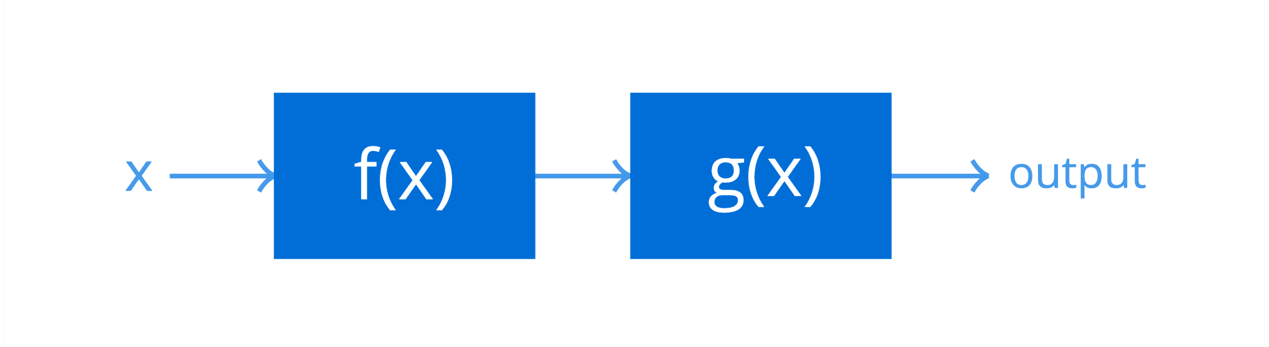
Consider two functions of a single independent variable, f(x) = 2x – 1 and g(x) = x3. Their composite function can be defined as follows:

h = g(f(x))

In this operation, g is a function of f. This means that g is applied to the result of applying the function, f, to x, producing h. 

Let’s consider a concrete example using the functions specified above to understand this better. 

Suppose that f(x) and g(x) are two systems in cascade, receiving an input x = 5:

Since f(x) is the first system in the cascade (because it is the inner function in the composite), its output is worked out first:

f(5) = (2 × 5) – 1 = 9

This result is then passed on as input to g(x), the second system in the cascade (because it is the outer function in the composite) to produce the net result of the composite function:

g(9) = 93 = 729

We could have, alternatively, computed the net result at one go, if we had performed the following computation:

h = g(f(x)) = (2x – 1)3 = 729

The composition of functions can also be considered as a chaining process, to use a more familiar term, where the output of one function feeds into the next one in the chain. 

With composite functions, the order matters. 

– Page 49, Calculus for Dummies, 2016.

Keep in mind that the composition of functions is a non-commutative process, which means that swapping the order of f(x) and g(x) in the cascade (or chain) does not produce the same results. Hence: 

g(f(x)) ≠ f(g(x))

The composition of functions can also be extended to the multivariate case:

h = g(r, s, t) = g(r(x, y), s(x, y), t(x, y)) = g(f(x, y)) 

Here, f(x, y) is a vector-valued function of two independent variables (or inputs), x and y. It is made up of three components (for this particular example) that are r(x, y), s(x, y) and t(x, y), and which are also known as the component functions of f.  

This means that f(x, y) will map two inputs to three outputs, and will then feed these three outputs into the consecutive system in the chain, g(r, s, t), to produce h. 

The Chain Rule

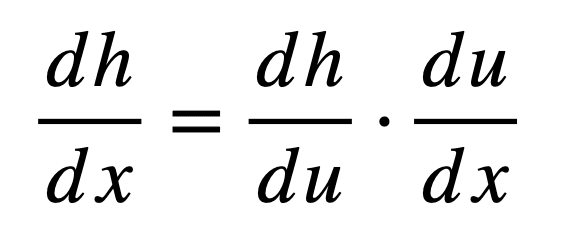
The chain rule allows us to find the derivative of a composite function. 

Let’s first define how the chain rule differentiates a composite function, and then break it into its separate components to understand it better. If we had to consider again the composite function, h = g(f(x)), then its derivative as given by the chain rule is:

Here, u is the output of the inner function f (hence, u = f(x)), which is then fed as input to the next function g to produce h (hence, h = g(u)). Notice, therefore, how the chain rule relates the net output, h, to the input, x, through an intermediate variable, u.

Recall that the composite function is defined as follows:

h(x) = g(f(x)) = (2x – 1)3

The first component of the chain rule, dh / du, tells us to start by finding the derivative of the outer part of the composite function, while ignoring whatever is inside. For this purpose, we shall apply the power rule:

((2x – 1)3)’ = 3(2x – 1)2

The result is then multiplied to the second component of the chain rule, du / dx, which is the derivative of the inner part of the composite function, this time ignoring whatever is outside:

( (2x – 1)’ )3 = 2

The derivative of the composite function as defined by the chain rule is, then, the following:

h’ = 3(2x – 1)2 × 2 = 6(2x – 1)2

We have, hereby, considered a simple example, but the concept of applying the chain rule to more complicated functions remains the same. We shall be considering more challenging functions in a separate tutorial. 

The Generalized Chain Rule

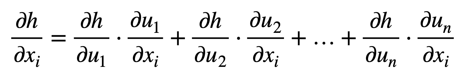
We can generalize the chain rule beyond the univariate case. 

Consider the case where x ∈ ℝm and u ∈ ℝn, which means that the inner function, f, maps m inputs to n outputs, while the outer function, g, receives n inputs to produce an output, h. For i = 1, …, m  the generalized chain rule states:

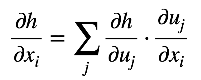
Or in its more compact form, for j = 1, …, n:

Recall that we employ the use of partial derivatives when we are finding the gradient of a function of multiple variables.

We can also visualize the workings of the chain rule by a tree diagram. 

Suppose that we have a composite function of two independent variables, x1 and x2, defined as follows:

h = g(f(x1, x2)) = g(u1(x1, x2), u2(x1, x2))

Here, u1 and u2 act as the intermediate variables. Its tree diagram would be represented as follows:

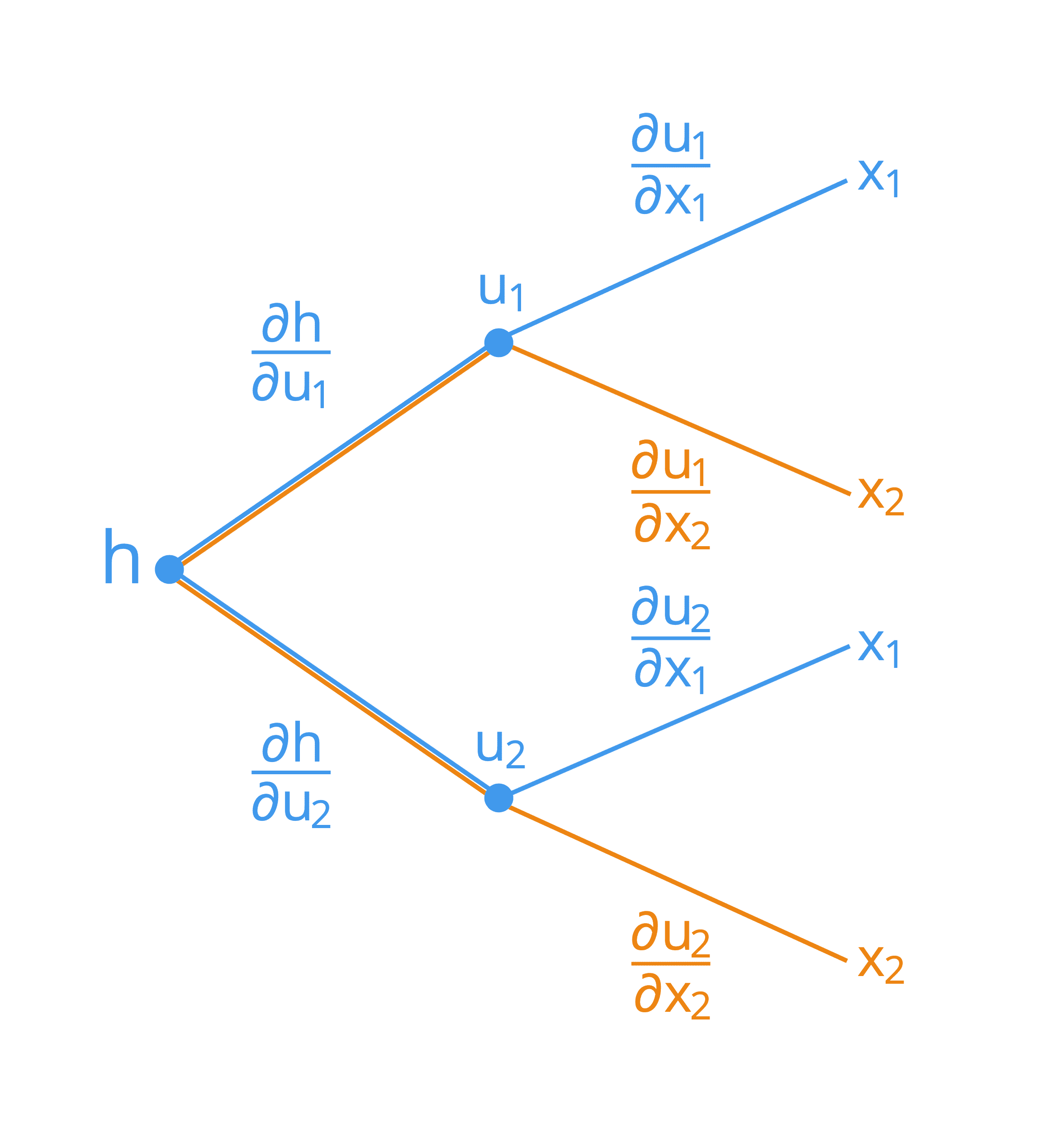
In order to derive the formula for each of the inputs, x1 and x2, we can start from the left hand side of the tree diagram, and follow its branches rightwards. In this manner, we find that we form the following two formulae (the branches being summed up have been colour coded for simplicity):

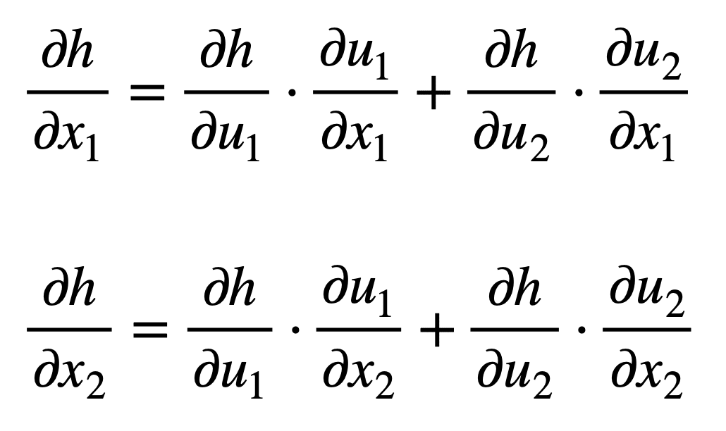
Notice how the chain rule relates the net output, h, to each of the inputs, xi, through the intermediate variables, uj. This is a concept that the backpropagation algorithm applies extensively to optimize the weights of a neural network.

Application in Machine Learning

Observe how similar the tree diagram is to the typical representation of a neural network (although we usually represent the latter by placing the inputs on the left hand side and the outputs on the right hand side). We can apply the chain rule to a neural network through the use of the backpropagation algorithm, in a very similar manner as to how we have applied it to the tree diagram above.

An area where the chain rule is used to an extreme is deep learning, where the function value y is computed as a many-level function composition. 

– Page 159, Mathematics for Machine Learning, 2020.

A neural network can, indeed, be represented by a massive nested composite function. For example:

y = fK ( fK – 1 ( … ( f1(x)) … ))

Here, x are the inputs to the neural network (for example, the images) whereas y are the outputs (for example, the class labels). Every function, fi, for i = 1, …, K, is characterized by its own weights. 

Applying the chain rule to such a composite function allows us to work backwards through all of the hidden layers making up the neural network, and efficiently calculate the error gradient of the loss function with respect to each weight, wi, of the network until we arrive to the input. 

Further Reading

This section provides more resources on the topic if you are looking to go deeper.

Books

Calculus for Dummies, 2016.
Single and Multivariable Calculus, 2020.
Deep Learning, 2017.
Mathematics for Machine Learning, 2020.

Summary

In this tutorial, you discovered the chain rule of calculus for univariate and multivariate functions.

Specifically, you learned:

A composite function is the combination of two (or more) functions. 
The chain rule allows us to find the derivative of a composite function.
The chain rule can be generalised to multivariate functions, and represented by a tree diagram. 
The chain rule is applied extensively by the backpropagation algorithm in order to calculate the error gradient of the loss function with respect to each weight.

Do you have any questions?
Ask your questions in the comments below and I will do my best to answer.

The post The Chain Rule of Calculus for Univariate and Multivariate Functions appeared first on Machine Learning Mastery.

Read MoreMachine Learning Mastery