Loss Functions in TensorFlow

Last Updated on July 15, 2022

Loss metric is very important for neural networks. As all machine learning model is a optimization problem or another, the loss is the objective function to minimize. In neural networks, the optimization is done with gradient descent and backpropagation. But what are loss functions and how are they affecting our neural networks?

In this post, we’ll cover what loss functions are and go into some commonly used loss functions and how you can apply them to your neural networks.

After reading this article, you will learn:

What are loss functions and how they are different from metrics
Common loss functions for regression and classification problems
How to use loss functions in your TensorFlow model

Let’s get started!

Overview

This article is split into five section; they are:

What are loss functions?
Mean absolute error
Mean squared error
Categorical cross-entropy
Loss functions in practice

What are loss functions?

In neural networks, loss functions help optimize the performance of the model. They are usually used to measure some penalty that the model is incurring on its predictions, such as the deviation of the prediction away from the ground truth label. Loss functions are usually differentiable across their domain (but it is allowed that the gradient is undefined only for very specific points, such as x = 0, which is basically ignored in practice). In the training loop, we differentiate them with respect to parameters and used these gradients for our backpropagation and gradient descent steps to optimize our model on the training set.

Loss functions are also slightly different from metrics. While loss functions can tell us the performance of our model, they might not be of direct interest or easily explainable by humans. This is where metrics come in. Metrics such as accuracy are much more useful for humans to understand the performance of a neural network even though they might not be good choices for loss functions since they might not be differentiable.

In the following, let’s explore some common loss functions, in particular, the mean absolute error, mean squared error, and categorical cross entropy.

Mean Absolute Error

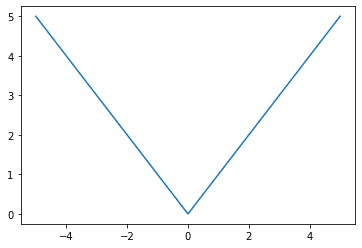
The mean absolute error (MAE) measures the absolute difference between predicted values and the ground truth labels and takes the mean of the difference across all training examples. Mathematically, it is equal to $frac{1}{m}sum_{i=1}^mlverthat{y}_i–y_irvert$ where $m$ is the number of training examples, $y_i$ and $hat{y}_i$ are the ground truth and predicted values respectively, and we are averaging over all training examples. The MAE is never negative, but it would be zero only if the prediction matched the ground truth perfectly. It is an intuitive loss function and might also be used as one of our metrics, in particular for regression problems since we would want to minimize the error in our predictions.

Let’s look at what the mean absolute error loss function looks like graphically:

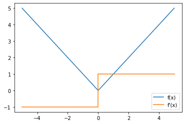
Similar to activation functions, we are usually also interested in what the gradient of the loss function looks like since we are using the gradient later on to do backpropagation to train our model’s parameters.

We notice that there is a discontinuity in the gradient function for the mean absolute loss function but we tend to ignore it since it occurs only at x = 0 which in practice rarely happens since it is the probability of a single point in a continuous distribution.

Let’s take a look at how to implement this loss function in TensorFlow using the the Keras losses module:

import tensorflow as tf
from tensorflow.keras.losses import MeanAbsoluteError

y_true = [1., 0.]
y_pred = [2., 3.]

mae_loss = MeanAbsoluteError()

print(mae_loss(y_true, y_pred).numpy())

which gives us 2.0 as the output as expected, since $ frac{1}{2}(lvert 2-1rvert + lvert 3-0rvert) = frac{1}{2}(4) = 4 $. Next, let’s explore another loss function for regression models with slightly different properties, the mean squared error.

Mean Squared Error

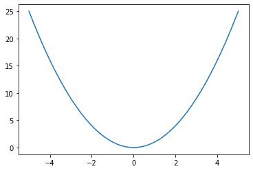
Another popular loss function for regression models is the mean squared error (MSE), which is equal to $frac{1}{m}sum_{i=1}^m(hat{y}_i–y_i)^2$. It is similar to the mean absolute error as it also measures the deviation of the predicted value from the ground truth value. However, the mean squared error squares this difference (always non-negative since square of real numbers are always non-negative), which gives it slightly different properties.

One notable one is that the mean squared error favors a large number of small errors over a small number of large errors, which leads to models that have less outliers or at least outliers that are less severe than models trained with a mean absolute error. This is because a large error would have a significantly larger impact on the error, and consequently the gradient of the error, when compared to a small error.

Graphically,

Then, looking at the gradient,

Notice that larger errors would lead to a larger magnitude for the gradient and also a larger loss. Hence, for example, two training examples that deviate from their ground truths by 1 unit would lead to a loss of 2, while a single training example that deviates from its ground truth by 2 units would lead to a loss of 4, hence having a larger impact.

Let’s look at how to implement the mean squared loss in TensorFlow.

import tensorflow as tf
from tensorflow.keras.losses import MeanSquaredError

y_true = [1., 0.]
y_pred = [2., 3.]

mse_loss = MeanSquaredError()

print(mse_loss(y_true, y_pred).numpy())

which gives the output 5.0 as expected since $frac{1}{2}[(2-1)^2 + (3-0)^2] = frac{1}{2}(10) = 5$. Notice that the second example with a predicted value of 3 and actual value of 0 contributes 90% of the error under the mean squared error vs 75% of the error under mean absolute error.

Sometimes, you may see people use root mean squared error (RMSE) as a metric. This is to take the square root of MSE. From the perspective of a loss function, MSE and RMSE are equivalent.

Both MAE and MSE are measuring values in a continuous range. Hence they are for regression problems. For classification problems, we can use categorical cross-entropy.

Categorical Cross-entropy

The previous two loss functions are for regression models, where the output could be any real number. However, for classification problems, there is a small, discrete set of numbers that the output could take. Furthermore, the number that we use to label-encode the classes are arbitrary, and with no semantic meaning (e.g. if we used the labels 0 for cat, 1 for dog, and 2 for horse, it does not represent that a dog is half cat and half horse). Therefore it should not have an impact on the performance of the model.

In a classification problem, the model’s output is a vector of probability for each category. In Keras models, usually we expect this vector to be “logits”, i.e., real numbers to be transformed to probability using softmax function, or the output of a softmax activation function.

The cross-entropy between two probability distributions is a measure of the difference between the two probability distributions. Precisely, it is $-sum_i P(X = x_i) log Q(X = x_i)$ for probability $P$ and $Q$. In machine learning, we usually have the probability $P$ provided by the training data and $Q$ predicted by the model, which $P$ is 1 for the correct class and 0 for every other class. The predicted probability $Q$, however, is usually valued between 0 and 1. Hence when used for classification problems in machine learning, this formula can be simplified into: $$text{categorical cross entropy} = – log p_{gt}$$ where $p_{gt}$ is the model-predicted probability of the ground truth class for that particular sample.

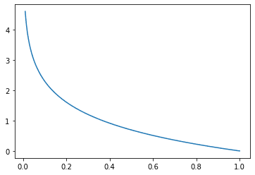
Cross-entropy metric have a negative sign because $log(x)$ tends to negative infinity as $x$ tends to zero. We want a higher loss when the probability approaches 0 and a lower loss when the probability approaches 1. Graphically,

Notice that the loss is exactly 0 if the probability of the ground truth class is 1 as desired. Also, as the probability of the ground truth class tends to 0, the loss tends to positive infinity as well, hence substantially penalizing bad predictions. You might recognize this loss function for logistic regression, and they are similar except the logistic regression loss is specific to the case of binary classes.

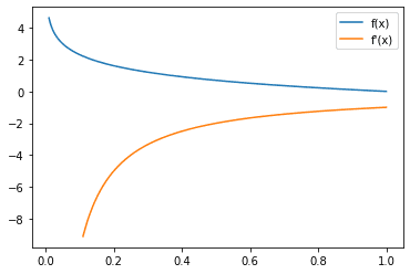
Now, looking at the gradient of the cross entropy loss,

Looking at the gradient, we can see that the gradient is generally negative which is also expected since to decrease this loss, we would want the probability on the ground truth class to be as high as possible, and recall that gradient descent goes in the opposite direction of the gradient.

There are two different ways to implement categorical cross entropy in TensorFlow. The first method takes in one-hot vectors as input,

import tensorflow as tf
from tensorflow.keras.losses import CategoricalCrossentropy

# using one hot vector representation
y_true = [[0, 1, 0], [1, 0, 0]]
y_pred = [[0.15, 0.75, 0.1], [0.75, 0.15, 0.1]]

cross_entropy_loss = CategoricalCrossentropy()

print(cross_entropy_loss(y_true, y_pred).numpy())

This gives the output as 0.2876821 which is equal to $-log(0.75)$ as expected. The other way of implementing the categorical cross entropy loss in TensorFlow is using a label-encoded representation for the class, where the class is represented by a single non-negative integer indicating the ground truth class instead.

import tensorflow as tf
from tensorflow.keras.losses import SparseCategoricalCrossentropy

y_true = [1, 0]
y_pred = [[0.15, 0.75, 0.1], [0.75, 0.15, 0.1]]

cross_entropy_loss = SparseCategoricalCrossentropy()

print(cross_entropy_loss(y_true, y_pred).numpy())

which likewise gives the output 0.2876821.

Now that we’ve explored loss functions for both regression and classification models, let’s take a look at how we use loss functions in our machine learning models.

Loss Functions in Practice

Let’s explore how we can use loss functions in practice. We’ll explore this through a simple dense model on the MNIST digit classification dataset.

First, we get the download the data from Keras datasets module,

import tensorflow.keras as keras

(trainX, trainY), (testX, testY) = keras.datasets.mnist.load_data()

Then, we build our model,

from tensorflow.keras import Sequential
from tensorflow.keras.layers import Dense, Input, Flatten

model = Sequential([
Input(shape=(28,28,1,)),
Flatten(),
Dense(units=84, activation=”relu”),
Dense(units=10, activation=”softmax”),
])

print (model.summary())

And we look at the model architecture outputted from the above code,

_________________________________________________________________
Layer (type) Output Shape Param #
=================================================================
flatten_1 (Flatten) (None, 784) 0

dense_2 (Dense) (None, 84) 65940

dense_3 (Dense) (None, 10) 850

=================================================================
Total params: 66,790
Trainable params: 66,790
Non-trainable params: 0
_________________________________________________________________

We can then compile our model, which is also where we introduce the loss function. Since this is a classification problem, we’ll use the cross entropy loss. In particular, since the MNIST dataset in Keras datasets is represented as a label instead of an one-hot vector, we’ll use the SparseCategoricalCrossEntropy loss.

model.compile(optimizer=”adam”, loss=tf.keras.losses.SparseCategoricalCrossentropy(), metrics=”acc”)

And finally, we train our model.

history = model.fit(x=trainX, y=trainY, batch_size=256, epochs=10, validation_data=(testX, testY))

And our model successfully trains with the following output:

Epoch 1/10
235/235 [==============================] – 2s 6ms/step – loss: 7.8607 – acc: 0.8184 – val_loss: 1.7445 – val_acc: 0.8789
Epoch 2/10
235/235 [==============================] – 1s 6ms/step – loss: 1.1011 – acc: 0.8854 – val_loss: 0.9082 – val_acc: 0.8821
Epoch 3/10
235/235 [==============================] – 1s 6ms/step – loss: 0.5729 – acc: 0.8998 – val_loss: 0.6689 – val_acc: 0.8927
Epoch 4/10
235/235 [==============================] – 1s 5ms/step – loss: 0.3911 – acc: 0.9203 – val_loss: 0.5406 – val_acc: 0.9097
Epoch 5/10
235/235 [==============================] – 1s 6ms/step – loss: 0.3016 – acc: 0.9306 – val_loss: 0.5024 – val_acc: 0.9182
Epoch 6/10
235/235 [==============================] – 1s 6ms/step – loss: 0.2443 – acc: 0.9405 – val_loss: 0.4571 – val_acc: 0.9242
Epoch 7/10
235/235 [==============================] – 1s 5ms/step – loss: 0.2076 – acc: 0.9469 – val_loss: 0.4173 – val_acc: 0.9282
Epoch 8/10
235/235 [==============================] – 1s 5ms/step – loss: 0.1852 – acc: 0.9514 – val_loss: 0.4335 – val_acc: 0.9287
Epoch 9/10
235/235 [==============================] – 1s 6ms/step – loss: 0.1576 – acc: 0.9577 – val_loss: 0.4217 – val_acc: 0.9342
Epoch 10/10
235/235 [==============================] – 1s 5ms/step – loss: 0.1455 – acc: 0.9597 – val_loss: 0.4151 – val_acc: 0.9344

And that’s one example of how to use a loss function in a TensorFlow model.

Further Reading

Below are the documentation of the loss functions from TensorFlow/Keras:

Mean absolute error: https://www.tensorflow.org/api_docs/python/tf/keras/losses/MeanAbsoluteError
Mean squared error: https://www.tensorflow.org/api_docs/python/tf/keras/losses/MeanSquaredError
Categorical cross entropy: https://www.tensorflow.org/api_docs/python/tf/keras/losses/CategoricalCrossentropy
Sparse categorical cross entropy: https://www.tensorflow.org/api_docs/python/tf/keras/losses/SparseCategoricalCrossentropy

Conclusion

In this post, you have seen loss functions and the role that they play in a neural network. You have also seen some popular loss functions used in regression and classification models, as well as how to use the cross entropy loss function in a TensorFlow model.

Specifically, you learned:

What are loss functions and how they are different from metrics
Common loss functions for regression and classification problems
How to use loss functions in your TensorFlow model

The post Loss Functions in TensorFlow appeared first on Machine Learning Mastery.

Read MoreMachine Learning Mastery