

The method of Lagrange multipliers is a simple and elegant method of finding the local minima or local maxima of a function subject to equality or inequality constraints. Lagrange multipliers are also called undetermined multipliers. In this tutorial we’ll talk about this method when given equality constraints.
In this tutorial, you will discover the method of Lagrange multipliers and how to find the local minimum or maximum of a function when equality constraints are present.
After completing this tutorial, you will know:
How to find points of local maximum or minimum of a function with equality constraints
Method of Lagrange multipliers with equality constraints
Let’s get started.
A Gentle Introduction To Method Of Lagrange Multipliers. Photo by Mehreen Saeed, some rights reserved.
Tutorial Overview
This tutorial is divided into 2 parts; they are:
Method of Lagrange multipliers with equality constraints
Two solved examples
Prerequisites
For this tutorial, we assume that you already know what are:
Derivative of functions
Function of several variables, partial derivatives and gradient vectors
A gentle introduction to optimization
Gradient descent
You can review these concepts by clicking on the links given above.
What Is The Method Of Lagrange Multipliers With Equality Constraints?
Suppose we have the following optimization problem:
Minimize f(x)
Subject to:
g_1(x) = 0
g_2(x) = 0
…
g_n(x) = 0
The method of Lagrange multipliers first constructs a function called the Lagrange function as given by the following expression.
L(x, 𝜆) = f(x) + 𝜆_1 g_1(x) + 𝜆_2 g_2(x) + … + 𝜆_n g_n(x)
Here 𝜆 represents a vector of Lagrange multipliers, i.e.,
𝜆 = [ 𝜆_1, 𝜆_2, …, 𝜆_n]^T
To find the points of local minimum of f(x) subject to the equality constraints, we find the stationary points of the Lagrange function L(x, 𝜆), i.e., we solve the following equations:
∇xL = 0
∂L/∂𝜆_i = 0 (for i = 1..n)
Hence, we get a total of m+n equations to solve, where
m = number of variables in domain of f
n = number of equality constraints.
In short, the points of local minimum would be the solution of the following equations:
∂L/∂x_j = 0 (for j = 1..m)
g_i(x) = 0 (for i = 1..n)
Solved Examples
This section contains two solved examples. If you solve both of them, you’ll get a pretty good idea on how to apply the method of Lagrange multipliers to functions of more than two variables, and a higher number of equality constraints.
Example 1: One Equality Constraint
Let’s solve the following minimization problem:
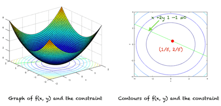
Minimize: f(x) = x^2 + y^2
Subject to: x + 2y – 1 = 0
The first step is to construct the Lagrange function:
L(x, y, 𝜆) = x^2 + y^2 + 𝜆(x + 2y – 1)
We have the following three equations to solve:
∂L/∂x = 0
2x + 𝜆 = 0 (1)
∂L/∂y = 0
2y + 2𝜆 = 0 (2)
∂L/∂𝜆 = 0
x + 2y -1 = 0 (3)
Using (1) and (2), we get:
𝜆 = -2x = -y
Plugging this in (3) gives us:
x = 1/5
y = 2/5
Hence, the local minimum point lies at (1/5, 2/5) as shown in the right figure. The left figure shows the graph of the function.
Example 2: Two Equality Constraints
Suppose we want to find the minimum of the following function subject to the given constraints:
minimize g(x, y) = x^2 + 4y^2
Subject to:
x + y = 0
x^2 + y^2 – 1 = 0
The solution of this problem can be found by first constructing the Lagrange function:
L(x, y, 𝜆_1, 𝜆_2) = x^2 + 4y^2 + 𝜆_1(x + y) + 𝜆_2(x^2 + y^2 – 1)
We have 4 equations to solve:
∂L/∂x = 0
2x + 𝜆_1 + 2x 𝜆_2 = 0 (1)
∂L/∂y = 0
8y + 𝜆_1 + 2y 𝜆_2 = 0 (2)
∂L/∂𝜆_1 = 0
x + y = 0 (3)
∂L/∂𝜆_2 = 0
x^2 + y^2 – 1 = 0 (4)
Solving the above system of equations gives us two solutions for (x,y), i.e. we get the two points:
(1/sqrt(2), -1/sqrt(2))
(-1/sqrt(2), 1/sqrt(2))
The function along with its constraints and local minimum are shown below.
Relationship to Maximization Problems
If you have a function to maximize, you can solve it in a similar manner, keeping in mind that maximization and minimization are equivalent problems, i.e.,
maximize f(x) is equivalent to minimize -f(x)
Importance Of The Method Of Lagrange Multipliers In Machine Learning
Many well known machine learning algorithms make use of the method of Lagrange multipliers. For example, the theoretical foundations of principal components analysis (PCA) are built using the method of Lagrange multipliers with equality constraints. Similarly, the optimization problem in support vector machines SVMs is also solved using this method. However, in SVMS, inequality constraints are also involved.
Extensions
This section lists some ideas for extending the tutorial that you may wish to explore.
Optimization with inequality constraints
KKT conditions
Support vector machines
If you explore any of these extensions, I’d love to know. Post your findings in the comments below.
Further Reading
This section provides more resources on the topic if you are looking to go deeper.
Tutorials
Derivatives
Gradient descent for machine learning
What is gradient in machine learning
Partial derivatives and gradient vectors
How to choose an optimization algorithm
Resources
Additional resources on Calculus Books for Machine Learning
Books
Thomas’ Calculus, 14th edition, 2017. (based on the original works of George B. Thomas, revised by Joel Hass, Christopher Heil, Maurice Weir)
Calculus, 3rd Edition, 2017. (Gilbert Strang)
Calculus, 8th edition, 2015. (James Stewart)
Summary
In this tutorial, you discovered what is the method of Lagrange multipliers. Specifically, you learned:
Lagrange multipliers and the Lagrange function
How to solve an optimization problem when equality constraints are given
Do you have any questions?
Ask your questions in the comments below and I will do my best to answer.
The post A Gentle Introduction To Method Of Lagrange Multipliers appeared first on Machine Learning Mastery.
Read MoreMachine Learning Mastery